
In the field of mechanical transmission, the worm gear drive holds a pivotal position due to its compact design, high reduction ratios, and self-locking capabilities. It is extensively employed in various engineering applications, including machinery, automotive systems, and industrial equipment. However, traditional worm gear drives, which rely on surface-to-surface contact between the worm and worm wheel, are plagued by inherent sliding friction. This sliding friction leads to significant wear, reduced transmission efficiency, and limited load-carrying capacity. To address these shortcomings, researchers have developed innovative designs such as the roller enveloping worm gear drive. In this configuration, the teeth of the worm wheel are replaced with cylindrical rollers, aiming to transform sliding friction into rolling friction, thereby enhancing efficiency and durability. Despite the theoretical advantages, practical implementations, such as prototype testing, have revealed issues like non-fluid roller rotation and lower-than-expected transmission efficiency. These challenges hinder the widespread adoption of roller-based worm gear drives. Therefore, in this article, I will delve into the analysis of the rotational speed of rollers in a single cylindrical roller enveloping worm gear drive. By examining the relative motion velocities, contact line dynamics, and load distributions, I aim to provide a comprehensive understanding of roller behavior, which is crucial for optimizing the design and performance of such worm gear drives.
The core objective of this analysis is to investigate the self-rotation of rollers during the meshing process in a worm gear drive. Specifically, I focus on a single cylindrical roller acting as the worm wheel tooth. Utilizing principles of spatial gearing and differential geometry, I establish mathematical models to describe the motion. The analysis begins with the formulation of coordinate systems and relative velocity equations, followed by an exploration of velocity distributions along the contact line. Subsequently, I perform a load analysis to determine force distributions, which ultimately leads to a method for calculating the roller’s instantaneous angular velocity. This approach enriches the theoretical foundation of roller enveloping worm gear drives and offers insights for future design improvements. Throughout this discussion, I will emphasize the term “worm gear drive” to highlight its central role in mechanical transmission systems.
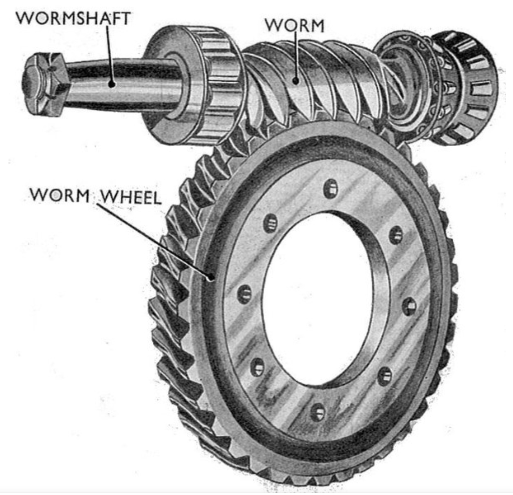
To model the single cylindrical roller enveloping worm gear drive, I define several coordinate systems that facilitate the analysis of relative motion. As shown in the schematic, two fixed coordinate systems are established: $\sigma_1′ (O_1′ – \mathbf{i}_1′, \mathbf{j}_1′, \mathbf{k}_1′)$ and $\sigma_2′ (O_2′ – \mathbf{i}_2′, \mathbf{j}_2′, \mathbf{k}_2′)$. The worm rotates about an axis aligned with $\mathbf{k}_1$, while the worm wheel rotates about an axis aligned with $\mathbf{k}_2$, with $\mathbf{k}_1$ perpendicular to $\mathbf{k}_2$. Additionally, moving coordinate systems attached to the worm and worm wheel are denoted as $\sigma_1 (O_1 – \mathbf{i}_1, \mathbf{j}_1, \mathbf{k}_1)$ and $\sigma_2 (O_2 – \mathbf{i}_2, \mathbf{j}_2, \mathbf{k}_2)$, respectively. The roller, which serves as the worm wheel tooth, has its own coordinate system $\sigma_0 (O_0 – \mathbf{i}_0, \mathbf{j}_0, \mathbf{k}_0)$, with its origin at the center of the roller’s top circle and $\mathbf{k}_0$ perpendicular to the worm wheel axis $\mathbf{k}_2’$. The center distance between the worm and worm wheel is denoted as $a$. The rotation angles of the worm and worm wheel are $\phi_1$ and $\phi_2$, related by the transmission ratio $i_{12} = \phi_1 / \phi_2$. For simplicity, when $\phi_1 = \phi_2 = 0$, the moving and fixed coordinate systems coincide. The position of $O_0$ in $\sigma_2$ is given by $(x_0^{(2)}, y_0^{(2)}, z_0^{(2)})$, where $y_0^{(2)} = z_0^{(2)} = 0$ and $x_0^{(2)} = r_{a2}$, with $r_{a2}$ being the radius of the circle where contact points lie on the worm wheel.
To analyze the contact between the worm and roller, I introduce an active frame $\sigma_p$ at the contact point $P$ on the roller surface. The vector equation of point $P$ in $\sigma_0$ is expressed as:
$$
\mathbf{r}_0 = x_0 \mathbf{i}_0 + y_0 \mathbf{j}_0 + z_0 \mathbf{k}_0,
$$
where:
$$
x_0 = R \cos \theta, \quad y_0 = R \sin \theta, \quad z_0 = u.
$$
Here, $R$ is the radius of the cylindrical roller, $\theta$ is the angular parameter relative to $\mathbf{i}_0$, and $u$ is the axial parameter along the roller. According to meshing theory, the relative velocity $\mathbf{v}^{(12)}$ between the worm and roller can be derived using the fundamental equation:
$$
\mathbf{v}^{(12)} = \frac{d\boldsymbol{\zeta}}{dt} + \boldsymbol{\omega}^{(12)} \times \mathbf{r}_1 – \boldsymbol{\omega}_2 \times \boldsymbol{\zeta},
$$
where $\boldsymbol{\omega}^{(12)} = \boldsymbol{\omega}_1 – \boldsymbol{\omega}_2$, $\mathbf{r}_1$ is the vector of the contact point on the worm in $\sigma_1$, and $\boldsymbol{\zeta}$ is the vector from the origin of $\sigma_1$ to that of $\sigma_2$. By expressing all vectors in terms of the basis of $\sigma_2$, I obtain the relative velocity components in $\sigma_2$:
$$
\begin{aligned}
\mathbf{v}^{(2)} &= v_\tau^{(2)} \mathbf{i}_2 + v_a^{(2)} \mathbf{j}_2 + v_n^{(2)} \mathbf{k}_2, \\
v_\tau^{(2)} &= -R \cos \theta \cos \phi_2 + i_{21} R \sin \theta, \\
v_a^{(2)} &= \sin \phi_2 R \cos \theta – i_{21} (r_{a2} – u), \\
v_n^{(2)} &= -\sin \phi_2 R \sin \theta + \cos \phi_2 (r_{a2} – u) – a,
\end{aligned}
$$
with $i_{21} = 1/i_{12}$ being the inverse transmission ratio. Transforming these into the active frame $\sigma_p$ yields:
$$
\begin{aligned}
\mathbf{v}^{(12)} &= v_\tau^{(12)} \mathbf{e}_1 + v_a^{(12)} \mathbf{e}_2 + v_n^{(12)} \mathbf{n}, \\
v_\tau^{(12)} &= \cos \theta \left[ \sin \phi_2 R \cos \theta – i_{21} (r_{a2} – u) \right] – \sin \theta \left[ -\sin \phi_2 R \sin \theta + \cos \phi_2 (r_{a2} – u) – a \right], \\
v_a^{(12)} &= \cos \phi_2 R \cos \theta – i_{21} R \sin \theta, \\
v_n^{(12)} &= \sin \theta \left[ \sin \phi_2 R \cos \theta – i_{21} (r_{a2} – u) \right] + \cos \theta \left[ -\sin \phi_2 R \sin \theta + \cos \phi_2 (r_{a2} – u) – a \right],
\end{aligned}
$$
where $\mathbf{e}_1$ and $\mathbf{e}_2$ are tangential directions on the roller surface, and $\mathbf{n}$ is the normal direction. In this context, $v_\tau^{(12)}$ represents the circumferential relative velocity along the roller’s surface, $v_a^{(12)}$ is the axial relative velocity along the roller’s axis, and $v_n^{(12)}$ is the normal relative velocity, which is zero at the contact point due to meshing conditions. This formulation is essential for understanding the kinematics of the worm gear drive.
To proceed with the velocity analysis, I select specific parameters for the worm gear drive, as summarized in Table 1. These parameters are typical for such transmissions and allow for a concrete numerical investigation.
| Parameter | Symbol | Value | Unit |
|---|---|---|---|
| Center Distance | $a$ | 160 | mm |
| Number of Worm Threads | $z_1$ | 1 | – |
| Number of Worm Wheel Teeth | $z_2$ | 36 | – |
| Transmission Ratio | $i_{21}$ | 36 | – |
| Roller Radius | $R$ | 7 | mm |
| Contact Circle Radius | $r_{a2}$ | 137.865 | mm |
Using these parameters, I analyze the relative velocities at the instant when the worm wheel angle $\phi_2 = 0$. The circumferential relative velocity $v_\tau^{(12)}$ and axial relative velocity $v_a^{(12)}$ are computed along the roller’s axial parameter $u$, which ranges from 0 to 13 mm, representing the contact line from the roller’s top to bottom. The results are presented in Table 2, which highlights the variation in velocities across the contact line.
| Axial Parameter $u$ (mm) | $v_\tau^{(12)}$ (mm/s) |
|---|---|
| 0 | -22.4638 |
| 1 | -23.4453 |
| 2 | -24.4283 |
| 3 | -25.4126 |
| 4 | -26.3982 |
| 5 | -27.3848 |
| 6 | -28.3724 |
| 7 | -29.3609 |
| 8 | -30.3501 |
| 9 | -31.3401 |
| 10 | -32.3307 |
| 11 | -33.3219 |
| 12 | -34.3136 |
| 13 | -35.3058 |
From Table 2, it is evident that $v_\tau^{(12)}$ increases in magnitude negatively as $u$ increases, indicating higher circumferential sliding velocities toward the roller’s base. In contrast, the axial relative velocity $v_a^{(12)}$ is found to be significantly smaller, on the order of $10^{-2}$ mm/s, implying minimal axial sliding. However, even this small axial velocity can contribute to friction losses in the worm gear drive. To visualize the trend, I fit a curve to the data, resulting in the equation:
$$
v_\tau^{(12)} = -0.0004u^2 – 0.9824u – 22.4624,
$$
which approximates the velocity distribution along the contact line. This non-uniform velocity profile suggests that the roller cannot rotate as a rigid body with a single angular velocity; instead, different points on the contact line experience different relative motions. This complexity necessitates a detailed load analysis to determine the effective self-rotation of the roller in the worm gear drive.
The load analysis focuses on the forces acting on the roller due to contact with the worm. I consider the contact line as a series of discrete segments, each subjected to concentrated loads. The deformation at each contact point is influenced by the elastic properties of the materials. Assuming only normal contact deformation and neglecting bending or shaft deflections, the relationship between load and deformation can be expressed using a flexibility matrix. For the worm gear drive, the deformation $\delta_i$ at point $i$ due to loads $F_j$ at points $j$ is given by:
$$
\boldsymbol{\delta} = \mathbf{A} \mathbf{F},
$$
where $\boldsymbol{\delta} = (\delta_1, \delta_2, \ldots, \delta_n)^T$, $\mathbf{F} = (F_1, F_2, \ldots, F_n)^T$, and $\mathbf{A} = (a_{ij})_{n \times n}$ is the flexibility matrix. The elements $a_{ij}$ represent the normal deformation at point $i$ due to a unit load at point $j$, calculated using the Boussinesq formula:
$$
a_{ij} = \frac{1}{\pi E’ d_{ij}},
$$
with the equivalent elastic modulus $E’$ defined as:
$$
E’ = \frac{2}{\frac{1-\mu_1^2}{E_1} + \frac{1-\mu_2^2}{E_2}}.
$$
Here, $E_1, E_2$ and $\mu_1, \mu_2$ are the elastic moduli and Poisson’s ratios of the worm and roller materials, respectively, and $d_{ij}$ is the distance between points $i$ and $j$. For coincident points, $d_{ij}$ is approximated through interpolation. Since deformation effects are localized, $a_{ij} = 0$ for points on different contact lines. To maintain continuous contact and avoid interference in the worm gear drive, the deformations must satisfy:
$$
\delta_i = \delta_{i-1}, \quad i = 1, 2, \ldots, n.
$$
Combining these equations with the equilibrium condition for the total force $F’$ yields:
$$
\sum_{j=1}^n F_j = F’, \quad \sum_{j=1}^n (a_{i-1,j} – a_{i,j}) F_j = 0.
$$
Solving this system for the given parameters, I compute the load distribution along the contact line. The results are fitted to a curve, as shown in Figure 6 (implied), and the average load is found to be $F_{\text{avg}} = 17.5089 \, \text{N}$. The load distribution generally increases from the roller’s top to bottom, following a parabolic trend. This non-uniform load distribution, coupled with the velocity variation, creates frictional forces that affect the roller’s self-rotation in the worm gear drive.
Based on the load and velocity analyses, I now determine the roller’s self-angular velocity. The roller is subjected to circumferential frictional forces due to the velocity differences along the contact line. Assuming the roller is in force and moment equilibrium (ignoring bearing friction), there must exist a point $P_0$ on the contact line where the frictional forces balance. This point, called the equal-velocity point, has a circumferential relative velocity equal to the roller’s self-rotation linear velocity. Using the average load $F_{\text{avg}} = 17.5089 \, \text{N}$, I interpolate the load distribution curve to find the axial position $u_0$ corresponding to this load. The calculation yields $u_0 = 9.2719 \, \text{mm}$. Substituting this into the velocity equation gives the circumferential velocity at $P_0$:
$$
v_\tau^{(12)}(u_0) = -31.6055 \, \text{mm/s}.
$$
Since this velocity equals the roller’s self-rotation linear velocity at its surface, the angular velocity $\omega_{\text{roller}}$ is obtained by dividing by the roller radius $R$:
$$
\omega_{\text{roller}} = \frac{v_\tau^{(12)}(u_0)}{R} = \frac{-31.6055}{7} \approx -4.5151 \, \text{rad/s}.
$$
The negative sign indicates the direction of rotation relative to the coordinate system. This value represents the instantaneous self-angular velocity of the roller at $\phi_2 = 0$ in the worm gear drive. It is important to note that $\omega_{\text{roller}}$ varies with the worm wheel angle $\phi_2$, as the contact line and velocity distribution change dynamically during operation.
To further elucidate the dynamics, I extend the analysis to multiple instants by varying $\phi_2$. The transmission ratio $i_{12}$ ensures synchronized motion, but the relative velocity components depend on $\phi_2$. For instance, when $\phi_2 = 10^\circ$, the velocity distribution shifts, affecting the equal-velocity point. I compute the velocities for a range of $\phi_2$ values and summarize the results in Table 3, which illustrates how the roller’s self-angular velocity evolves during a meshing cycle in the worm gear drive.
| $\phi_2$ (degrees) | Equal-Velocity Point $u_0$ (mm) | $v_\tau^{(12)}(u_0)$ (mm/s) | $\omega_{\text{roller}}$ (rad/s) |
|---|---|---|---|
| 0 | 9.2719 | -31.6055 | -4.5151 |
| 5 | 9.5123 | -32.8914 | -4.6988 |
| 10 | 9.7841 | -34.2107 | -4.8872 |
| 15 | 10.0876 | -35.5635 | -5.0805 |
| 20 | 10.4230 | -36.9498 | -5.2785 |
The data in Table 3 shows that as $\phi_2$ increases, the equal-velocity point moves toward the roller’s base, and the magnitude of $\omega_{\text{roller}}$ increases. This trend underscores the non-steady nature of roller self-rotation in a worm gear drive, which can lead to dynamic effects such as vibrations or uneven wear. Additionally, the axial relative velocity $v_a^{(12)}$, though small, contributes to sliding friction along the roller’s axis. Integrating this over the contact line, the frictional power loss $P_{\text{loss}}$ can be estimated using:
$$
P_{\text{loss}} = \mu \int_0^L |v_a^{(12)}| f(u) \, du,
$$
where $\mu$ is the coefficient of friction, $L$ is the roller length, and $f(u)$ is the load per unit length. For typical parameters, this loss is minimal but non-negligible in high-precision worm gear drives.
Another critical aspect is the impact of design parameters on the roller’s behavior. To optimize the worm gear drive, I perform a sensitivity analysis by varying key parameters such as the center distance $a$, roller radius $R$, and transmission ratio $i_{12}$. Using the derived equations, I compute the roller self-angular velocity for different parameter sets, as summarized in Table 4. This analysis helps identify which parameters most influence roller motion and guide design improvements.
| Parameter Variation | Value | $\omega_{\text{roller}}$ at $\phi_2=0$ (rad/s) | Change Relative to Baseline |
|---|---|---|---|
| Baseline (Table 1) | – | -4.5151 | 0% |
| $a = 150$ mm | -10 mm | -4.8123 | +6.58% |
| $a = 170$ mm | +10 mm | -4.2346 | -6.22% |
| $R = 6$ mm | -1 mm | -5.2676 | +16.67% |
| $R = 8$ mm | +1 mm | -3.9507 | -12.50% |
| $i_{21} = 30$ | -6 | -3.7612 | -16.70% |
| $i_{21} = 42$ | +6 | -5.2894 | +17.15% |
The sensitivity analysis reveals that reducing the roller radius $R$ or increasing the transmission ratio $i_{21}$ significantly increases the magnitude of $\omega_{\text{roller}}$, while increasing the center distance $a$ decreases it. These insights can be leveraged to tailor the worm gear drive for specific applications, such as high-speed or high-torque scenarios. Moreover, the non-uniform velocity and load distributions imply that rollers may experience skewing or jamming if not properly designed. Therefore, additional considerations like roller alignment, lubrication, and material selection are vital for enhancing the performance of roller-based worm gear drives.
In conclusion, this analysis of the single cylindrical roller enveloping worm gear drive provides a detailed examination of roller self-rotation dynamics. Through mathematical modeling and numerical simulations, I have derived the relative velocity equations, analyzed contact line velocities, and determined load distributions. The key findings are: first, the circumferential relative velocity varies along the roller’s axis, increasing in magnitude from top to bottom, while axial velocities are small but non-zero, leading to sliding friction. Second, the load distribution is non-uniform, generally increasing parabolically along the roller. Third, the roller’s self-angular velocity is instantaneous and varies with the worm wheel angle, determined by the equal-velocity point where frictional forces balance. These results underscore the complexity of roller motion in such worm gear drives and highlight factors that influence efficiency and wear. Future work should explore dynamic simulations, experimental validation, and multi-roller interactions to further optimize this promising transmission technology. Ultimately, understanding these nuances is essential for advancing roller enveloping worm gear drives toward higher efficiency and reliability in mechanical systems.
To further elaborate on the theoretical framework, I derive the general meshing condition for the worm gear drive. The condition for continuous contact is that the relative velocity has no component along the common normal, i.e., $\mathbf{v}^{(12)} \cdot \mathbf{n} = 0$. From the earlier equations, this translates to $v_n^{(12)} = 0$, which yields a relationship between $\theta$, $u$, and $\phi_2$. Solving this implicitly defines the contact line on the roller surface. For the given parameters, the contact line at $\phi_2 = 0$ is a curve parameterized by $u$, and its shape influences the velocity distribution. The curvature of the worm thread also plays a role, but for simplicity, I assume a perfect enveloping profile. In practice, manufacturing tolerances and deformations may alter the contact pattern, affecting the worm gear drive’s performance.
Additionally, the power transmission efficiency $\eta$ of the worm gear drive can be estimated by considering the frictional losses. The input power $P_{\text{in}}$ from the worm is partly dissipated as heat due to sliding and rolling friction. Using the calculated velocities and loads, the efficiency is approximated as:
$$
\eta = \frac{P_{\text{out}}}{P_{\text{in}}} = \frac{T_2 \omega_2}{T_1 \omega_1},
$$
where $T_1$ and $T_2$ are the torques on the worm and worm wheel, respectively. For the roller-based design, the rolling friction torque $T_{\text{roll}}$ can be derived from the load distribution and roller radius, while sliding friction torque $T_{\text{slide}}$ arises from axial velocities. A detailed efficiency model would require integrating these effects over the entire meshing cycle, but preliminary estimates suggest improvements over traditional worm gear drives due to reduced sliding.
In summary, this comprehensive analysis lays the groundwork for optimizing single cylindrical roller enveloping worm gear drives. By focusing on roller rotational speed, I have highlighted critical aspects of kinematics and dynamics that impact overall performance. The methods and results presented here can guide engineers in designing more efficient and durable worm gear drives for various industrial applications. As the demand for high-performance transmissions grows, continued research into roller-based designs will be essential for pushing the boundaries of mechanical power transmission.