
I study the assembly process of hypoid bevel gears because these gears occupy a critical position in the rear drive axle main reducer of an automobile. The meshing performance of hypoid bevel gears determines the stability of power transmission, the level of transmission noise, and the overall NVH behavior of the vehicle. In my work, I treat meshing performance as a combination of two measurable responses: the amplitude of transmission error and the position, shape, and size of the tooth contact pattern. Both responses are affected by manufacturing deviations and by installation errors introduced during assembly. In many previous studies, theoretical tooth surfaces are used in simulation while actual gears are used in rolling tests, which creates an inconsistent evaluation standard. To avoid this inconsistency, I reconstruct real tooth surfaces and use them as the basis for finite element simulation, contact pattern prediction, and assembly process optimization.
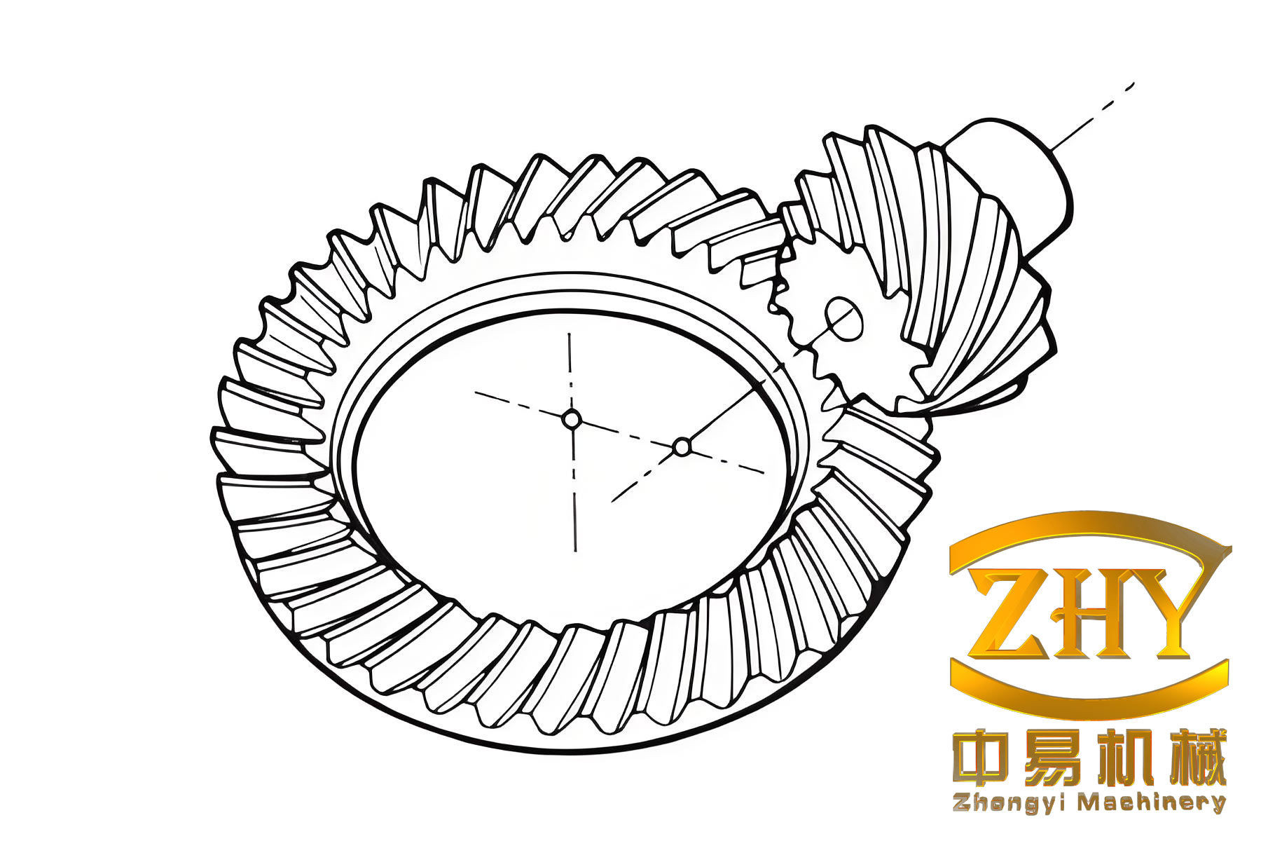
My starting point is the kinematic and conjugate meshing theory of hypoid bevel gears. I model the two tooth surfaces as regular parameterized surfaces. If the driving gear surface is \(\Sigma_1\) and the driven gear surface is \(\Sigma_2\), then each surface can be written as
$$
\mathbf{r}^{(i)}=\mathbf{r}^{(i)}(u_i,\theta_i),\qquad
\mathbf{r}_{u_i}^{(i)}\times \mathbf{r}_{\theta_i}^{(i)}\neq \mathbf{0},
\qquad i=1,2 .
$$
The unit normal vector of each surface is
$$
\mathbf{n}^{(i)}=
\frac{\mathbf{r}_{u_i}^{(i)}\times \mathbf{r}_{\theta_i}^{(i)}}
{\left\|\mathbf{r}_{u_i}^{(i)}\times \mathbf{r}_{\theta_i}^{(i)}\right\|},
\qquad i=1,2 .
$$
For a conjugate pair of hypoid bevel gears, the two surfaces must satisfy both position continuity and normal continuity at the instantaneous contact point. I write this condition in a fixed reference frame as
$$
\begin{cases}
\mathbf{r}_{h}^{(1)}(u_1,\theta_1,\phi_1)=
\mathbf{r}_{h}^{(2)}(u_2,\theta_2,\phi_2),\\[4pt]
\mathbf{n}_{h}^{(1)}(u_1,\theta_1,\phi_1)=
\mathbf{n}_{h}^{(2)}(u_2,\theta_2,\phi_2).
\end{cases}
$$
Because the contact is tangential and continuous, the relative velocity must be perpendicular to the common normal. This gives the meshing equation
$$
\mathbf{n}\cdot \mathbf{V}=0 .
$$
I use this equation to solve for the instantaneous contact point. If the initial contact point is known, the contact trace can be obtained by introducing the rotation angles of the two members and solving the nonlinear system with a Newton iteration method. In this way, I can describe the contact path on the real tooth surface instead of only on an ideal theoretical surface. The contact point and contact trace calculations are essential for hypoid bevel gears because the final contact pattern is directly related to the assembly position.
The main installation errors that I consider are the offset error \(\Delta V\), the pinion axial mounting distance error \(\Delta H\), the gear axial mounting distance error \(\Delta E\), and the shaft angle error \(\Delta \Sigma\). These errors are unavoidable in the assembly of hypoid bevel gears. The offset error changes the relative position of the two axes in the offset direction. The pinion axial mounting distance error changes the axial position of the driving gear. The gear axial mounting distance error changes the axial position of the driven gear. The shaft angle error changes the angle between the two axes. I summarize the notation and the typical adjustment range in the following table.
| Installation error | Symbol | Physical meaning | Typical range |
|---|---|---|---|
| Offset error | \(\Delta V\) | Deviation of the pinion axis from its theoretical offset position | \(-0.06\) to \(+0.06\) mm |
| Pinion axial mounting distance error | \(\Delta H\) | Axial displacement of the pinion along its own axis | \(-0.06\) to \(+0.06\) mm |
| Gear axial mounting distance error | \(\Delta E\) | Axial displacement of the gear along its own axis | \(-0.06\) to \(+0.06\) mm |
| Shaft angle error | \(\Delta \Sigma\) | Angular deviation between the two gear axes | \(-0.06^\circ\) to \(+0.06^\circ\) |
For hypoid bevel gears, the transmission error is defined as the difference between the actual rotation angle of the driven gear and its theoretical rotation angle for a given rotation of the driving gear. I express it as
$$
TE=\phi_2(\phi_1)-\phi_2′(\phi_1)
=
\left(\phi_2-\phi_2^{(0)}\right)
–
\frac{z_1}{z_2}
\left(\phi_1-\phi_1^{(0)}\right),
$$
where \(z_1\) and \(z_2\) are the tooth numbers of the pinion and the gear, respectively, and \(\phi_1^{(0)}\) and \(\phi_2^{(0)}\) are the initial rotation angles. The transmission error curve of hypoid bevel gears is periodic, and its amplitude is one of the most important indicators of meshing quality. A large transmission error amplitude usually means stronger vibration and noise, while a small amplitude usually means smoother motion. However, a small transmission error alone is not sufficient because the contact pattern must also remain within the standard area.
The contact pattern of hypoid bevel gears is usually inspected by applying a marking compound to the tooth surface and rolling the pair under a light load. The area where the marking compound is removed indicates the contact region. Common defects include toe contact, heel contact, root contact, tip contact, wide contact, narrow contact, bridge-shaped contact, and diagonal contact. These defects appear when the tooth surface deviation and installation error shift the contact area away from the desired central region. Therefore, I quantify the contact pattern using distances from the tooth boundaries and the contact length in both the tooth height and tooth length directions.
Before reconstructing the real tooth surface, I need accurate measurement data. I use a gear measuring center to measure discrete points on the actual tooth surface. The theoretical tooth surface is first imported as a reference surface, and then a measurement grid is planned on the real tooth surface. I use a nine-by-five grid, which gives forty-five measurement points. The grid is arranged so that the tooth length direction is divided into nine columns and the tooth height direction is divided into five rows. This distribution is dense enough to capture the curvature variation of hypoid bevel gears while keeping the measurement time reasonable.
The measurement path is planned to reduce interference between the probe and the adjacent teeth. I choose a point-by-point measurement path that moves from one end of the tooth surface to the other. This path keeps the rotary table rotating in a consistent direction during measurement and reduces the influence of angular positioning errors. For the pinion, the probe is arranged to avoid collision with the neighboring tooth surfaces. For the gear, because the tooth surface is wider and the curvature is smaller, the probe can be arranged in a more direct orientation. I also apply probe radius compensation. If the measured center coordinate is \(\mathbf{r}_i\), the actual surface point \(\mathbf{R}_i\) is
$$
\mathbf{R}_i=\mathbf{r}_i \pm \mathbf{n}\,r,
$$
where \(\mathbf{n}\) is the unit normal at the corresponding point and \(r\) is the probe radius. This step is necessary because the measuring center records the center of the probe sphere rather than the physical contact point on the tooth surface.
After obtaining the real surface points, I reconstruct the tooth surface using non-uniform rational B-spline curves and surfaces. The NURBS curve is written as
$$
p(u)=
\frac{\sum_{i=0}^{n}\omega_i N_{i,k}(u)d_i}
{\sum_{i=0}^{n}\omega_i N_{i,k}(u)},
$$
where \(\omega_i\) are weights, \(d_i\) are control points, and \(N_{i,k}(u)\) are B-spline basis functions. The basis functions are defined recursively by
$$
N_{i,0}(u)=
\begin{cases}
1, & u_i\le u \le u_{i+1},\\
0, & \text{otherwise},
\end{cases}
$$
$$
N_{i,k}(u)=
\frac{u-u_i}{u_{i+k}-u_i}N_{i,k-1}(u)
+
\frac{u_{i+k+1}-u}{u_{i+k+1}-u_{i+1}}N_{i+1,k-1}(u).
$$
For cubic NURBS curves, I use the matrix form
$$
p_i(u)=\frac{U N_i D_i}{U N_i W_i},
\qquad 0\le u\le 1,
$$
where \(U=[1\ u\ u^2\ u^3]\), \(N_i\) is the cubic basis matrix, \(D_i\) contains weighted control points, and \(W_i\) contains the weights. I use accumulated chord length parameterization to determine the node vector. The node vector is important because it controls how the measured points are distributed along the curve. For an open curve, I set the first and last node multiplicities to four so that the curve passes through the end points and the end tangent directions are retained.
The NURBS surface is generated by a bicubic formulation. The surface equation is
$$
p(u,v)=
\frac{
\sum_{i=0}^{m}\sum_{j=0}^{n}
B_{i,k}(u)B_{j,l}(v)\omega_{i,j}d_{i,j}
}{
\sum_{i=0}^{m}\sum_{j=0}^{n}
B_{i,k}(u)B_{j,l}(v)\omega_{i,j}
}.
$$
I first fit curves in one parameter direction to obtain intermediate control points, and then fit curves in the other parameter direction to obtain the final control grid. This procedure is repeated for the pinion and the gear. After the control grid is obtained, I import it into a CAD environment and generate the reconstructed real tooth surface. The reconstructed surfaces are then used to build the three-dimensional models of the hypoid bevel gears.
To verify the accuracy of the reconstruction, I compare the fitted surface with the theoretical reference surface at the same grid locations. The maximum normal deviation is kept below \(0.1\,\mu\text{m}\). This level of accuracy is sufficient for meshing simulation because the deviation is much smaller than the assembly adjustment resolution and the contact pattern sensitivity. I summarize the reconstruction accuracy in the following table.
| Region | Maximum normal deviation | Acceptance criterion |
|---|---|---|
| Pinion convex surface | Less than \(0.1\,\mu\text{m}\) | Satisfied |
| Pinion concave surface | Less than \(0.1\,\mu\text{m}\) | Satisfied |
| Gear convex surface | Less than \(0.1\,\mu\text{m}\) | Satisfied |
| Gear concave surface | Less than \(0.1\,\mu\text{m}\) | Satisfied |
Once the real tooth surface models are established, I import them into finite element analysis software. I use a mesh generation tool to discretize the hypoid bevel gears. The mesh is refined on the contacting tooth surfaces and coarsened on the non-contacting regions. This strategy improves computational efficiency while maintaining enough resolution in the contact zone. The material properties are assigned as elastic modulus \(E=212000\,\text{MPa}\), Poisson ratio \(\nu=0.3\), and density \(\rho=7.8\times 10^3\,\text{kg/m}^3\). I define the contact as a surface-to-surface contact with a penalty formulation and a friction coefficient of \(0.1\). The driving gear is controlled to rotate about its own axis, and a torque is applied to the driven gear. The boundary conditions and analysis steps are summarized below.
| Item | Setting |
|---|---|
| Contact type | Surface-to-surface contact |
| Master surface | Pinion tooth surface |
| Slave surface | Gear tooth surface |
| Contact formulation | Penalty method |
| Sliding formulation | Finite sliding |
| Friction coefficient | 0.1 |
| Driving motion | Angular velocity on the pinion |
| Load | Torque on the gear |
I first compare the transmission error obtained from a theoretical tooth surface model and from a real tooth surface model. When all installation errors are zero, the theoretical model gives a transmission error that is nearly centered at zero, but the real tooth surface model gives a constant offset and a larger fluctuation. This difference confirms that manufacturing deviations exist in the actual hypoid bevel gears and that a theoretical model cannot fully represent the actual meshing behavior. The comparison is summarized in the following table.
| Model type | Mean transmission error | Amplitude of fluctuation |
|---|---|---|
| Theoretical tooth surface | Close to \(0\) | Relatively small |
| Real reconstructed tooth surface | About \(2.5\times 10^{-3}\,\text{rad}\) | Relatively large |
Next, I study the influence of a single installation error on the transmission error of hypoid bevel gears. I change one error at a time while keeping the other errors zero. The offset error \(\Delta V\) shifts the transmission error curve in the positive direction as \(\Delta V\) increases. When \(\Delta V\) is positive, the fluctuation amplitude changes more noticeably. The pinion axial mounting distance error \(\Delta H\) shifts the transmission error curve in the negative direction as \(\Delta H\) increases. A positive \(\Delta H\) can make the fluctuation smoother, but a negative \(\Delta H\) makes the offset more obvious. The gear axial mounting distance error \(\Delta E\) mainly changes the backlash and has only a small effect on the transmission error amplitude. The shaft angle error \(\Delta \Sigma\) changes the overall level of the transmission error and also causes strong fluctuation when its magnitude increases.
I quantify the sensitivity of the transmission error to each installation error. The sensitivity order I obtain is
$$
\Delta \Sigma=\Delta H>\Delta V>\Delta E .
$$
This means that the shaft angle error and the pinion axial mounting distance error are the most important factors for transmission error control in hypoid bevel gears. The offset error is also important, especially when it is positive. The gear axial mounting distance error has the weakest influence. I summarize the single-error effects in the following table.
| Installation error | Main effect on transmission error | Sensitivity rank |
|---|---|---|
| \(\Delta V\) | Shifts the curve and changes fluctuation when positive | 3 |
| \(\Delta H\) | Shifts the curve and changes fluctuation strongly | 1 |
| \(\Delta E\) | Mainly changes backlash, weak effect on amplitude | 4 |
| \(\Delta \Sigma\) | Changes the overall level and causes strong fluctuation | 1 |
I verify the simulation results with rolling tests. I set the offset error to \(\pm 0.04\,\text{mm}\), the pinion axial mounting distance error to \(\pm 0.04\,\text{mm}\), and the shaft angle error to \(\pm 4\) arc seconds. I compare the transmission error amplitude from the theoretical model, the real reconstructed model, and the actual produced hypoid bevel gears. The results show that the real reconstructed model is much closer to the actual rolling test than the theoretical model. This confirms that using real tooth surfaces in simulation is reasonable and reliable. The comparison for the offset error is shown below.
| Error case | Theoretical model amplitude | Real reconstructed model amplitude | Actual gear amplitude |
|---|---|---|---|
| \(\Delta V=+0.04\,\text{mm}\) | \(8.420\,\mu\text{rad}\) | \(10.870\,\mu\text{rad}\) | \(11.399\,\mu\text{rad}\) |
| \(\Delta V=-0.04\,\text{mm}\) | \(10.710\,\mu\text{rad}\) | \(13.280\,\mu\text{rad}\) | \(12.712\,\mu\text{rad}\) |
For the pinion axial mounting distance error, the real reconstructed model again follows the actual gear more closely than the theoretical model. The same conclusion holds for the shaft angle error. This is important because it shows that the real tooth surface reconstruction reduces the evaluation mismatch between simulation and experiment for hypoid bevel gears.
| Error case | Theoretical model amplitude | Real reconstructed model amplitude | Actual gear amplitude |
|---|---|---|---|
| \(\Delta H=+0.04\,\text{mm}\) | \(12.390\,\mu\text{rad}\) | \(16.510\,\mu\text{rad}\) | \(17.252\,\mu\text{rad}\) |
| \(\Delta H=-0.04\,\text{mm}\) | \(19.780\,\mu\text{rad}\) | \(21.330\,\mu\text{rad}\) | \(20.902\,\mu\text{rad}\) |
| Error case | Theoretical model amplitude | Real reconstructed model amplitude | Actual gear amplitude |
|---|---|---|---|
| \(\Delta \Sigma=+4”\) | \(5.710\,\mu\text{rad}\) | \(6.860\,\mu\text{rad}\) | \(6.803\,\mu\text{rad}\) |
| \(\Delta \Sigma=-4”\) | \(4.770\,\mu\text{rad}\) | \(6.820\,\mu\text{rad}\) | \(6.798\,\mu\text{rad}\) |
After studying single installation errors, I investigate the combined effect of the offset error and the pinion axial mounting distance error. In actual assembly of hypoid bevel gears, the shaft angle error is usually controlled within a very small tolerance, and the gear axial mounting distance error is difficult to adjust and has a weak influence. Therefore, I focus on \(\Delta V\) and \(\Delta H\). I choose nine combinations. The simulation shows that when \(\Delta H\) is in the range from \(0\) to \(+0.04\,\text{mm}\) and \(\Delta V\) is in the range from \(-0.06\) to \(0\,\text{mm}\), the two errors partially cancel each other and produce a smaller constant offset. When \(\Delta H\) is greater than \(+0.04\,\text{mm}\) and \(\Delta V\) is negative, the two errors reinforce each other and produce a larger offset. The amplitude results are summarized below.
| \(\Delta H\) (mm) | \(\Delta V=-0.02\) mm | \(\Delta V=-0.04\) mm | \(\Delta V=-0.06\) mm |
|---|---|---|---|
| \(0.02\) | \(11.6\,\mu\text{rad}\) | \(11.3\,\mu\text{rad}\) | \(6.7\,\mu\text{rad}\) |
| \(0.04\) | \(10.3\,\mu\text{rad}\) | \(9.6\,\mu\text{rad}\) | \(7.4\,\mu\text{rad}\) |
| \(0.06\) | \(2.8\,\mu\text{rad}\) | \(2.5\,\mu\text{rad}\) | \(2.9\,\mu\text{rad}\) |
Although the transmission error amplitude can be reduced by choosing a particular combination of \(\Delta V\) and \(\Delta H\), the contact pattern must also be checked. A small transmission error does not guarantee that the contact pattern lies in the standard region. For hypoid bevel gears, the contact pattern is evaluated by four geometric parameters: the minimum distance from the contact area to the toe boundary, the maximum contact length in the tooth length direction, the minimum distance from the contact area to the tip boundary, and the maximum contact length in the tooth height direction. I denote these parameters as \(A\), \(B\), \(C\), and \(H\). The required ranges are given in the following table.
| Parameter | Meaning | Required range | Preferred ratio |
|---|---|---|---|
| \(A\) | Distance from contact area to toe in tooth length direction | \(5.38\) to \(12.90\,\text{mm}\) | \(1/6\) to \(1/2.5\) of tooth width |
| \(B\) | Maximum contact length in tooth length direction | \(12.92\) to \(21.51\,\text{mm}\) | \(1/2.5\) to \(1/1.5\) of tooth width |
| \(C\) | Distance from contact area to tip in tooth height direction | \(1.26\) to \(2.21\,\text{mm}\) | \(1/7\) to \(1/4\) of tooth height |
| \(H\) | Maximum contact length in tooth height direction | \(2.94\) to \(4.41\,\text{mm}\) | \(1/3\) to \(1/2\) of tooth height |
I define an objective function to optimize the contact pattern of hypoid bevel gears. If \(A_0\), \(B_0\), \(C_0\), and \(H_0\) are the preferred values, and \(A_x\), \(B_x\), \(C_x\), and \(H_x\) are the deviations caused by installation errors, then the objective is to minimize
$$
F_{\min}=
k_a(A_0+A_x)^2+
k_b(B_0+B_x)^2+
k_c(C_0+C_x)^2+
k_d(H_0+H_x)^2 .
$$
The weighting coefficients \(k_a\), \(k_b\), \(k_c\), and \(k_d\) are introduced because the four parameters have different units and different sensitivities. The installation errors must remain within their adjustable ranges:
$$
\begin{cases}
V_1\le V\le V_2,\\
H_1\le H\le H_2,\\
E_1\le E\le E_2,\\
\Sigma_1\le \Sigma\le \Sigma_2 .
\end{cases}
$$
Because the objective function is not an explicit function of the installation errors, I use a golden section search method. This method is suitable for single-variable and multi-variable optimization when the function is evaluated numerically. I first determine a descending interval, then choose a golden ratio point, and then iteratively reduce the interval until the convergence condition is satisfied. The golden ratio point is computed as
$$
c=a+0.618034(b-a).
$$
The convergence condition is
$$
\frac{|b-d|}{|c-a|}<\varepsilon,
$$
where \(\varepsilon\) is a small tolerance. I apply this method to optimize the installation errors so that the contact pattern of hypoid bevel gears remains within the standard region while the transmission error stays in a controllable range.
As an example, I start from a random installation error combination and adjust \(\Delta V\) and \(\Delta H\). The initial values and the optimized values are listed below. The adjustment is small, but it moves the contact pattern toward the preferred area without increasing the transmission error beyond the allowed limit.
| Item | \(\Delta V\) (mm) | \(\Delta H\) (mm) | Adjustment |
|---|---|---|---|
| Initial | \(-0.023\) | \(0.035\) | — |
| Optimized | \(-0.012\) | \(-0.015\) | \(\Delta V=0.011,\ \Delta H=-0.050\) |
I verify the optimized contact pattern by rolling the actual hypoid bevel gears. The contact marks on the gear convex surface and the pinion concave surface agree well with the simulation. This agreement shows that the real reconstructed tooth surface model is accurate and that the golden section search method is effective for contact pattern optimization. It also shows that the contact pattern and transmission error can be used together as evaluation criteria for the assembly of hypoid bevel gears.
I then move to the assembly process of the main reducer. The main reducer consists of a differential assembly and a main reducer subassembly. The differential assembly contains side gears, pinion gears, spherical washers, and a differential housing. The main reducer subassembly contains the driving pinion, the driven gear, bearings, spacers, seals, and a housing. During assembly, the pinion mounting distance is adjusted by selecting a shim thickness. The offset error is determined by the housing machining quality. I use statistical process control to monitor the offset distance of the housing, and the offset error is usually kept within \(0.02\,\text{mm}\). The relationship between the housing dimension \(L_1\), the shim thickness \(e\), the standard mounting distance \(H\), and the pinion axial mounting distance error \(\Delta H\) is
$$
L_1=\Delta H+H+e .
$$
For the studied main reducer, the standard mounting distance is \(92\,\text{mm}\). After measuring the housing, I obtain an offset error of \(\Delta V=-0.015\,\text{mm}\). I then use the real reconstructed tooth surface model to simulate five sets of hypoid bevel gears. The target transmission error range is from \(8\,\mu\text{rad}\) to \(14\,\mu\text{rad}\), because this range corresponds to acceptable NVH behavior in the vehicle. The first optimization step gives the following results.
| Main reducer set | 1 | 2 | 3 | 4 | 5 |
|---|---|---|---|---|---|
| Transmission error amplitude (\(\mu\text{rad}\)) | \(9.71\) | \(12.59\) | \(8.33\) | \(11.66\) | \(10.73\) |
| \(\Delta H\) (mm) | \(0.038\) | \(0.027\) | \(0.043\) | \(0.019\) | \(0.016\) |
These results show that the transmission error can be kept inside the desired range by adjusting the pinion axial mounting distance error. However, I still need to ensure that the contact pattern is standard. Therefore, I use the contact pattern objective function and the golden section search method again. The initial values come from the transmission error optimization. The optimized values, the selected shim thickness, and the final transmission error amplitude are given below.
| Main reducer set | 1 | 2 | 3 | 4 | 5 |
|---|---|---|---|---|---|
| Initial \(\Delta V\) (mm) | \(-0.015\) | \(-0.015\) | \(-0.015\) | \(-0.015\) | \(-0.015\) |
| Initial \(\Delta H\) (mm) | \(0.038\) | \(0.027\) | \(0.043\) | \(0.019\) | \(0.016\) |
| Optimized \(\Delta V\) (mm) | \(0.0011\) | \(0.0020\) | \(0.0050\) | \(0.0045\) | \(0.0230\) |
| Optimized \(\Delta H\) (mm) | \(-0.008\) | \(-0.006\) | \(-0.026\) | \(-0.022\) | \(-0.009\) |
| Shim thickness (mm) | \(1.382\) | \(1.277\) | \(1.336\) | \(1.259\) | \(1.295\) |
| Final transmission error amplitude (\(\mu\text{rad}\)) | \(10.63\) | \(9.55\) | \(7.58\) | \(12.71\) | \(8.94\) |
The rolling tests show that the contact pattern of the hypoid bevel gears is located in the standard region and that the transmission error remains within the controllable interval. The experimental contact marks on both the convex and concave surfaces are consistent with the simulation. This confirms that the assembly process optimization method is reliable. By using real tooth surfaces, finite element simulation, and contact pattern optimization, I can avoid excessive reliance on manual experience when selecting shim thicknesses. The assembly quality of hypoid bevel gears becomes more repeatable, and the assembly efficiency improves.
I also compare the final assembly results with the acceptance criteria. The transmission error amplitude of all five sets remains below \(14\,\mu\text{rad}\), and the contact pattern stays inside the required ranges for \(A\), \(B\), \(C\), and \(H\). The main reducer noise behavior is therefore expected to meet the target. The method I propose connects real tooth surface measurement, NURBS reconstruction, finite element simulation, sensitivity analysis, contact pattern optimization, and assembly shim selection into a single workflow for hypoid bevel gears.
| Evaluation item | Acceptance criterion | Result |
|---|---|---|
| Transmission error amplitude | \(8\) to \(14\,\mu\text{rad}\) | All five sets satisfied |
| Contact pattern position | Within standard tooth length and height ranges | Satisfied |
| Contact pattern shape | No severe toe, heel, root, tip, or diagonal defect | Satisfied |
| Shim thickness selection | Calculated from assembly relation | Satisfied |
In my research, the most important conclusion is that real tooth surface reconstruction greatly improves the reliability of simulation for hypoid bevel gears. A theoretical tooth surface model may predict a small transmission error, but the actual hypoid bevel gears have manufacturing deviations that produce a larger transmission error. When I use the reconstructed real tooth surface, the simulation results match the rolling test results closely. This allows me to use simulation with confidence for assembly optimization.
Another conclusion is that the shaft angle error and the pinion axial mounting distance error are the most influential installation errors for the transmission error of hypoid bevel gears. The offset error is also important, especially when it is positive. The gear axial mounting distance error has the weakest influence. Therefore, during assembly, I prioritize the control of \(\Delta \Sigma\) and \(\Delta H\), then \(\Delta V\), and finally \(\Delta E\). This priority helps reduce the transmission error amplitude efficiently.
I also conclude that transmission error and contact pattern must be optimized together. If only the transmission error is minimized, the contact pattern may move away from the standard region and cause uneven load distribution, which can reduce the service life of hypoid bevel gears. If only the contact pattern is controlled, the transmission error may become too large and produce noise and vibration. By combining both criteria, I obtain an assembly scheme that satisfies both smooth motion and acceptable contact behavior.
The golden section search method is suitable for this problem because the objective function is evaluated numerically and the installation errors have bounded ranges. The method converges quickly and provides a practical adjustment for \(\Delta V\) and \(\Delta H\). In the assembly of hypoid bevel gears, the adjustment is realized by selecting the proper shim thickness. The assembly relation \(L_1=\Delta H+H+e\) links the simulation result directly to the physical shim. This makes the optimization result easy to apply on the assembly line.
For future work, I plan to extend the method to include contact stress and loaded contact analysis. The contact stress distribution on hypoid bevel gears is also important for fatigue life and load capacity. I also plan to include vehicle-level NVH testing so that the relationship between transmission error, contact pattern, and vehicle noise can be evaluated more directly. In addition, I would like to study the influence of tooth surface roughness and heat treatment deformation on the real tooth surface reconstruction. These factors may further improve the accuracy of the simulation model for hypoid bevel gears.
Overall, I have developed a systematic approach for the assembly optimization of hypoid bevel gears based on real tooth surfaces. The approach includes measurement planning, NURBS curve and surface fitting, CAD model generation, finite element simulation, installation error sensitivity analysis, contact pattern optimization, and assembly shim calculation. The experimental validation shows that the method is reliable and that it can improve the assembly quality and efficiency of the main reducer. The method is especially useful for hypoid bevel gears because their meshing performance is highly sensitive to installation errors and tooth surface deviations. By using real tooth surfaces and optimizing both transmission error and contact pattern, I can achieve a more stable, quieter, and more durable transmission.