
I investigate the coupled thermal, metallurgical, mechanical, and manufacturing behavior of thin-web aviation gears made of 9310 steel. My central concern is the residual stress and distortion that develop during carburizing, quenching, tempering, deep cryogenic treatment, and the subsequent gear cutting operation. In particular, I treat gear cutting after heat treatment as a critical stage because the initial residual stress field inherited from heat treatment interacts strongly with the cutting-induced thermal and mechanical loads. This interaction changes the final tooth geometry, web flatness, surface integrity, and fatigue performance. I therefore build a multi-field simulation framework that connects heat treatment with post-heat gear cutting and uses orthogonal experiments, range analysis, and grey relational analysis to optimize the process parameters.
The thin-web geometry is efficient for aviation transmission systems because it reduces mass while maintaining load capacity. However, the same geometry amplifies distortion sensitivity. During carburizing and quenching, the web and the teeth cool at different rates, transform at different times, and experience incompatible volume changes. During gear cutting, the tool removes a thin layer from the web, releasing part of the inherited stress and introducing new machining stress. The final state is not simply the sum of two independent processes. I model it as an inherited and evolving field problem. My approach includes the carburizing field, hardness field, temperature field, microstructure field, stress-strain field, cutting temperature, cutting force, machining residual stress, and final deformation.
For the carburizing field, I begin from Fick’s second law. Carbon diffuses into the austenite matrix under a concentration gradient. The three-dimensional diffusion equation I use is
$$ \frac{\partial C}{\partial t} = D \left( \frac{\partial^2 C}{\partial x^2} + \frac{\partial^2 C}{\partial y^2} + \frac{\partial^2 C}{\partial z^2} \right) $$
where \(C\) is carbon concentration, \(t\) is time, \(x\), \(y\), and \(z\) are spatial coordinates, and \(D\) is the carbon diffusion coefficient. The boundary condition follows Fick’s first law and is written as
$$ -D \frac{\partial C}{\partial n} = \beta (C_g – C_s) $$
with
$$ \beta = \beta_0 \exp\left(-\frac{E}{RT}\right) $$
In my model, \(C_g\) is the gas carbon potential, \(C_s\) is the surface carbon concentration, \(\beta\) is the carbon transfer coefficient, \(E\) is the activation energy, \(R\) is the gas constant, and \(T\) is the absolute temperature. I use a temperature-dependent and composition-dependent diffusion coefficient. The alloying elements modify the carbon activity and diffusivity. The empirical form I adopt is
$$ D(C,T) = 0.0047 \exp\left(-\frac{37000 – 6600C}{RT}\right) \exp(1.6C) q $$
where \(q\) is an alloy influence factor. For 9310 steel, I calculate \(q\) from the alloy composition and obtain a value of approximately 0.5886. At 900 °C, this gives a diffusion coefficient on the order of \(1.4 \times 10^{-5}\,\text{mm}^2/\text{s}\). This value is important because it controls the case depth during gear cutting preparation and later influences the hardness gradient, phase transformation, and residual stress after gear cutting.
The hardness field is not an independent variable. I derive it from the volume fractions of the phases and their individual hardness values. The rule I use is
$$ H_e = \sum V_{fi} H_i $$
where \(H_e\) is the equivalent hardness, \(V_{fi}\) is the volume fraction of phase \(i\), and \(H_i\) is the hardness of phase \(i\). For martensite, pearlite, ferrite, and bainite, I use composition-sensitive empirical expressions. For martensite, the Vickers hardness is approximated by
$$ HV_M = 127 + 949C + 27Si + 11Mn + 8Ni + 16Cr + 21\log V $$
For ferrite and pearlite mixtures, I use a coupled expression that depends on carbon, silicon, manganese, nickel, chromium, molybdenum, vanadium, and the volume fractions of ferrite and pearlite. For bainite, I use another composition-dependent relation. These expressions allow me to predict the hardness gradient from the surface to the core after carburizing and quenching. The hardness gradient is essential because the hard case and tough core produce a strong residual stress profile, which then affects gear cutting stability and final distortion.
For the temperature field, I solve the transient heat conduction equation with a phase-change latent heat term:
$$ \rho C_p \frac{\partial T}{\partial t} = \lambda \left( \frac{\partial^2 T}{\partial x^2} + \frac{\partial^2 T}{\partial y^2} + \frac{\partial^2 T}{\partial z^2} \right) + q_v $$
Here \(\rho\) is density, \(C_p\) is specific heat, \(\lambda\) is thermal conductivity, and \(q_v\) is the latent heat released or absorbed by phase transformation. The boundary condition at the gear surface follows Newton’s law of cooling:
$$ -\lambda \frac{\partial T}{\partial n} = h(T – T_f) $$
where \(h\) is the convective heat transfer coefficient and \(T_f\) is the medium temperature. I apply different \(h\) values for heating, air cooling, oil quenching, and deep cryogenic treatment. These boundary conditions control the temperature gradient, which in turn controls thermal stress, phase transformation sequence, and distortion.
For phase transformation kinetics, I separate diffusion-controlled transformation from diffusionless martensitic transformation. For diffusion-controlled transformation, I use the Johnson-Mehl-Avrami-Kolmogorov form:
$$ \xi = 1 – \exp(-b t^n) $$
where \(\xi\) is the transformed volume fraction, \(b\) is a rate constant, and \(n\) is the Avrami exponent. I obtain the transformation start and finish temperatures from the continuous cooling or isothermal transformation behavior of 9310 steel. For austenite decomposition into ferrite, pearlite, and bainite, I use a simplified kinetic form:
$$ \xi_J = 1 – \exp\left[ -A \left( \frac{T – T_s}{T_e – T_s} \right)^D \right] $$
For martensite, the transformation is temperature-dependent and quasi-athermal. I use
$$ \xi_M = 1 – \exp\left[ \psi_1 T + \psi_2 C + \psi_3 \sigma_m + \psi_4 \sigma_e + \psi_5 \right] $$
In the stress-free condition, the mean stress and equivalent stress terms vanish. Using the martensite start and finish temperatures for 9310 steel at different carbon levels, I obtain the material constants \(\psi_1 = 0.020413\), \(\psi_2 = 6.213\), and \(\psi_4 = -7.7304\). These constants allow me to predict how the carbon gradient produced by carburizing shifts the martensite start temperature from the surface to the core. This shift is one reason why the core transforms before the carburized surface during quenching.
For the stress-strain field, I use a thermo-elastoplastic constitutive relation that includes elastic strain, plastic strain, thermal strain, transformation strain, and transformation plasticity. The total strain increment is
$$ d\varepsilon_{ij} = d\varepsilon_{ij}^{e} + d\varepsilon_{ij}^{p} + d\varepsilon_{ij}^{th} + d\varepsilon_{ij}^{tr} + d\varepsilon_{ij}^{tp} $$
The thermal strain increment is
$$ d\varepsilon_{ij}^{th} = \sum_{k=1}^{5} m_k \alpha_k dT $$
The transformation strain increment is
$$ d\varepsilon_{ij}^{tr} = \sum_{k=1}^{5} V_k \beta_k^T $$
The elastic strain increment follows Hooke’s law with temperature-dependent Young’s modulus and Poisson’s ratio:
$$ d\varepsilon_{ij}^{e} = \frac{1+\nu}{E} d\sigma_{ij} – \frac{\nu}{E} d\sigma_{kk} $$
The plastic strain increment follows the associated flow rule:
$$ d\varepsilon_{ij}^{p} = \frac{3}{2} \frac{d\sigma_i}{H} \frac{s_{ij}}{\sigma_i} $$
The transformation plasticity increment is
$$ d\varepsilon_{ij}^{tp} = 3 K_{ij} (1 – V) dV $$
These equations are solved together with the temperature and phase fields. Because the material properties depend strongly on temperature and phase state, I build a material database from experiments and thermodynamic calculation.
| Element | C | Ni | Cr | Mo | Mn | Si | B |
|---|---|---|---|---|---|---|---|
| Mass fraction (%) | 0.11 | 3.35 | 1.21 | 0.08 | 0.53 | 0.23 | ≤0.001 |
I measured the thermal physical properties and mechanical properties of 9310 steel over a wide temperature range. The following table summarizes the measured data used in my heat treatment simulation and gear cutting simulation.
| Temperature (°C) | Young’s modulus (GPa) | Specific heat (J·g⁻¹·K⁻¹) | Thermal conductivity (W·m⁻¹·K⁻¹) | Thermal expansion (10⁻⁶ K⁻¹) | Thermal diffusivity (mm²·s⁻¹) | Poisson’s ratio |
|---|---|---|---|---|---|---|
| 25 | 221.256 | 0.434 | 22.368 | 10.415 | 6.701 | 0.291 |
| 100 | 218.274 | 0.471 | 23.607 | 11.654 | 6.517 | 0.293 |
| 200 | 212.178 | 0.500 | 24.192 | 12.743 | 6.291 | 0.294 |
| 300 | 206.658 | 0.525 | 24.241 | 13.717 | 6.003 | 0.301 |
| 400 | 193.542 | 0.561 | 25.309 | 14.305 | 5.635 | 0.304 |
| 500 | 187.657 | 0.642 | 26.351 | 14.718 | 5.134 | 0.307 |
| 600 | 176.275 | 0.686 | 24.680 | 15.023 | 4.488 | 0.310 |
| 700 | 166.654 | 0.894 | 23.273 | 15.144 | 3.546 | 0.314 |
| 800 | 161.772 | 0.827 | 24.464 | 15.206 | 4.542 | 0.321 |
| 900 | 152.698 | 0.785 | 25.548 | 15.225 | 5.588 | 0.325 |
| 1000 | 147.354 | 0.724 | 26.138 | 15.290 | 5.692 | 0.331 |
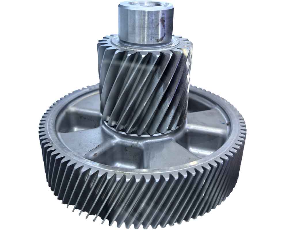
The gear I study is a thin-web aviation gear with module 2.5 mm, 92 teeth, face width 7 mm, and pressure angle 20°. I create the three-dimensional geometry and then refine the tooth region with hexahedral elements. The carburized surface is limited to the tooth flanks, while the non-carburized regions are protected. The heat treatment route includes carburizing, air cooling, high-temperature tempering, austenitizing, oil quenching, deep cryogenic treatment, low-temperature tempering, and final air cooling. The route is summarized below.
| Stage | Temperature | Atmosphere or medium | Time |
|---|---|---|---|
| Heating | 800 °C | Furnace | Controlled ramp |
| Boost carburizing | 900 °C | Carbon potential 1.3% | 4 h |
| Diffusion carburizing | 880 °C | Carbon potential 1.1% | 4 h |
| Air cooling | 25 °C | Air | To room temperature |
| High-temperature tempering | 650 °C | Furnace | 4 h |
| Austenitizing | 820 °C | Furnace | 4 h |
| Oil quenching | 60 °C | Oil | 0.5 h |
| Deep cryogenic treatment | −60 °C | Liquid nitrogen atmosphere | 3.5 h |
| Low-temperature tempering | 200 °C | Furnace | 4 h |
| Final cooling | 25 °C | Air | To room temperature |
After the heat treatment model is solved, I extract the residual stress field from the web and map it into the post-heat gear cutting model. This mapping is a key step because gear cutting after carburizing and quenching does not begin from a stress-free blank. The web carries a complex initial stress state. I sample the stress distribution along the web thickness direction and apply the averaged values to corresponding element layers in a two-dimensional orthogonal cutting model. The cutting model uses a plane strain assumption, a rigid tool, a rake angle of 10°, a clearance angle of 10°, CPE4RT elements, and a predefined stress field. The tool material is TiAlN-coated carbide with the properties listed below.
| Tool property | Value |
|---|---|
| Young’s modulus | 510 GPa |
| Specific heat | 0.975 J·g⁻¹·K⁻¹ |
| Thermal conductivity | 10 W·m⁻¹·K⁻¹ |
| Thermal expansion | 7.24 × 10⁻⁶ K⁻¹ |
| Density | 4545 kg·m⁻³ |
| Poisson’s ratio | 0.331 |
For the gear cutting simulation, I use the Johnson-Cook constitutive model because it captures strain hardening, strain-rate sensitivity, and thermal softening. The flow stress is
$$ \sigma = \left( A + B \varepsilon^n \right) \left( 1 + C \ln \frac{\dot{\varepsilon}}{\dot{\varepsilon}_0} \right) \left[ 1 – \left( \frac{T – T_r}{T_m – T_r} \right)^m \right] $$
The parameters I use for 9310 steel are \(A = 1000\) MPa, \(B = 800\) MPa, \(C = 0.014\), \(n = 0.25\), and \(m = 1.03\). For chip separation, I use the Johnson-Cook damage model:
$$ \varepsilon_f = \left( D_1 + D_2 \exp\left( D_3 \frac{p}{q} \right) \right) \left( 1 + D_4 \ln \frac{\dot{\varepsilon}}{\dot{\varepsilon}_0} \right) \left( 1 + D_5 T^* \right) $$
The damage parameter is
$$ D = \sum \frac{\Delta \varepsilon}{\varepsilon_f} $$
When \(D\) reaches 1, the element is deleted and the chip separates from the workpiece. The damage constants I use are \(D_1 = 0.00625\), \(D_2 = 0.65\), \(D_3 = 2.12\), \(D_4 = 0.002\), and \(D_5 = 0\). The contact friction is modeled with a mixed Coulomb and shear friction law:
$$ \tau_f = \mu \sigma_n, \quad \tau_f \le k $$
$$ \tau_f = k, \quad \tau_f > k $$
This friction law is necessary for accurate prediction of cutting force, cutting temperature, and residual stress during gear cutting. The thermal and mechanical loads in gear cutting are concentrated near the tool edge and the rake face. The primary deformation zone produces severe shear, the secondary deformation zone produces sliding and sticking friction, and the tertiary deformation zone produces surface burnishing and residual stress.
I first analyze the heat treatment results. The carbon concentration after carburizing decreases from the surface to the core. The effective case depth is defined either at 0.4% carbon or at 52 HRC. The tooth tip has the largest case depth, followed by the pitch region and the root region. The reason is that the tooth tip is convex, exposed, and thin, so it heats faster and receives more carbon. The root is concave, thicker, and partly shielded, so carbon diffusion is slower. The measured and simulated carbon gradients are summarized below.
| Location | Effective carburized depth at 0.4% C (mm) | Effective hardened depth at 52 HRC (mm) |
|---|---|---|
| Tooth tip | 0.96 | 0.92 |
| Pitch circle | 0.88 | 0.85 |
| Tooth root | 0.78 | 0.73 |
I use orthogonal experiments to optimize the carburizing stage. The objective is to maximize the effective case depth at the tooth root because the root fillet is a fatigue-critical region. I select four factors: boost time, boost carbon potential, diffusion time, and diffusion carbon potential. The factor levels are listed below.
| Level | Boost time (h) | Boost carbon potential (%) | Diffusion time (h) | Diffusion carbon potential (%) |
|---|---|---|---|---|
| 1 | 3 | 1.2 | 3 | 0.9 |
| 2 | 4 | 1.3 | 4 | 1.0 |
| 3 | 5 | 1.4 | 5 | 1.1 |
The orthogonal array and the resulting root case depth are listed below.
| Run | Boost time (h) | Boost carbon potential (%) | Diffusion time (h) | Diffusion carbon potential (%) | Root case depth (mm) |
|---|---|---|---|---|---|
| 1 | 3 | 1.2 | 3 | 0.9 | 0.715 |
| 2 | 3 | 1.3 | 4 | 1.0 | 0.864 |
| 3 | 3 | 1.4 | 5 | 1.1 | 0.893 |
| 4 | 4 | 1.2 | 4 | 1.1 | 0.851 |
| 5 | 4 | 1.3 | 5 | 0.9 | 0.839 |
| 6 | 4 | 1.4 | 3 | 1.0 | 0.842 |
| 7 | 5 | 1.2 | 5 | 1.0 | 0.913 |
| 8 | 5 | 1.3 | 3 | 1.1 | 0.895 |
| 9 | 5 | 1.4 | 4 | 0.9 | 0.902 |
The range analysis of the carburizing stage gives the following results. The influence order is boost time, diffusion time, diffusion carbon potential, and boost carbon potential. The optimal combination for maximum root case depth is boost time 5 h, boost carbon potential 1.4%, diffusion time 5 h, and diffusion carbon potential 1.1%. With this combination, the root case depth reaches 0.94 mm.
| Factor | Level 1 average | Level 2 average | Level 3 average | Range |
|---|---|---|---|---|
| Boost time | 0.824 | 0.844 | 0.903 | 0.079 |
| Boost carbon potential | 0.826 | 0.866 | 0.879 | 0.053 |
| Diffusion time | 0.817 | 0.872 | 0.882 | 0.065 |
| Diffusion carbon potential | 0.819 | 0.873 | 0.880 | 0.061 |
During quenching, the temperature field evolves rapidly. At the beginning of quenching, the surface cools much faster than the core. The tooth tip is the first region to lose heat, while the core remains hot. As quenching continues, the core also cools, and the temperature difference first increases and then decreases. After 500 s, the entire gear reaches the oil temperature. The temperature history confirms that the tooth tip has the highest cooling rate, the root has an intermediate cooling rate, and the core has the lowest cooling rate. This non-uniform cooling is the origin of thermal stress and distortion.
| Quenching time (s) | Maximum temperature (°C) | Minimum temperature (°C) | Maximum difference (°C) |
|---|---|---|---|
| 0 | 820.00 | 820.00 | 0.00 |
| 0.5 | 818.62 | 449.84 | 368.78 |
| 5 | 555.89 | 339.00 | 216.89 |
| 20 | — | — | 106.22 |
| 50 | — | — | 77.91 |
| 500 | 60.00 | 60.00 | 0.00 |
The microstructure evolution shows a clear carbon effect. The core, with lower carbon content, has a higher martensite start temperature and transforms first. The carburized surface, with higher carbon content, has a lower martensite start temperature and transforms later. In my simulation, the core begins martensitic transformation at about 5 s, while the tooth tip and root begin at about 50 s. At the end of transformation, the core retains about 5.1% austenite and forms about 94.1% martensite. The tooth tip retains about 11.2% austenite and forms about 84.6% martensite. The root retains about 9.4% austenite and forms about 86.7% martensite. This difference in transformation timing and volume change is a major source of residual stress and distortion.
| Location | Martensite start time (s) | Final martensite (%) | Final retained austenite (%) |
|---|---|---|---|
| Tooth tip | ≈50 | 84.6 | 11.2 |
| Tooth root | ≈50 | 86.7 | 9.4 |
| Core | ≈5 | 94.1 | 5.1 |
The tangential residual stress evolution is complex. At the very beginning of quenching, the surface cools and contracts, while the core remains hot. The surface is constrained by the core, so it tends to develop tensile stress, while the core develops compressive stress. As the core cools and contracts more than the surface, the surface stress becomes compressive and the core stress becomes tensile. When the core transforms to martensite first, it expands, reversing the sign again. Finally, when the carburized surface transforms, it expands and creates a compressive stress at the surface and a tensile stress in the core. The final residual stress state is compressive at the surface and tensile in the core. The tooth root reaches a compressive stress of about −417.4 MPa under the optimized quenching condition.
The displacement evolution follows a sequence of expansion, contraction, re-expansion, and re-contraction. The radial displacement and axial displacement both change sign during quenching. At the end of quenching, the tooth tip has a radial expansion of about 0.214 mm under the optimized condition, and the axial displacement is about 0.071 mm. The tooth root and core show smaller but non-negligible displacements. The thin web is especially sensitive to axial displacement because even a small amount of warpage changes the web flatness and later affects gear cutting allowances.
I optimize the quenching stage using a second orthogonal experiment. The factors are high-temperature tempering temperature, holding time, quenching temperature, and deep cryogenic treatment time. The responses are radial displacement, axial displacement, and tangential residual stress. Because these responses have different units, I normalize them and use a weighted composite score. The weights are 0.4 for radial displacement, 0.2 for axial displacement, and 0.4 for tangential stress. The normalization formula is
$$ S = 100 \frac{X_{\text{actual}} – X_{\text{worst}}}{X_{\text{best}} – X_{\text{worst}}} $$
and the composite score is
$$ S_{\text{total}} = 0.4 S_r + 0.2 S_a + 0.4 S_s $$
The quenching factor levels are listed below.
| Level | High-temperature tempering temperature (°C) | Holding time (h) | Quenching temperature (°C) | Deep cryogenic time (h) |
|---|---|---|---|---|
| 1 | 600 | 3 | 40 | 2 |
| 2 | 650 | 4 | 60 | 4 |
| 3 | 700 | 5 | 80 | 6 |
The orthogonal results and composite scores are summarized below.
| Run | Tempering temperature (°C) | Holding time (h) | Quenching temperature (°C) | Cryogenic time (h) | Radial displacement (mm) | Axial displacement (mm) | Tangential stress (MPa) | Composite score |
|---|---|---|---|---|---|---|---|---|
| 1 | 600 | 3 | 40 | 2 | 0.2697 | 0.0757 | −544.656 | 59.220 |
| 2 | 600 | 4 | 60 | 4 | 0.3208 | 0.0909 | −428.367 | 38.273 |
| 3 | 600 | 5 | 80 | 6 | 0.3286 | 0.0922 | −388.855 | 41.189 |
| 4 | 650 | 3 | 60 | 6 | 0.3206 | 0.0926 | −457.256 | 29.840 |
| 5 | 650 | 4 | 80 | 2 | 0.3283 | 0.0922 | −400.534 | 38.516 |
| 6 | 650 | 5 | 40 | 4 | 0.2698 | 0.0741 | −551.456 | 58.905 |
| 7 | 700 | 3 | 80 | 4 | 0.3277 | 0.0945 | −391.180 | 40.580 |
| 8 | 700 | 4 | 40 | 6 | 0.2690 | 0.0736 | −535.744 | 63.797 |
| 9 | 700 | 5 | 60 | 2 | 0.3205 | 0.0932 | −460.772 | 28.492 |
The range analysis of the composite score gives the influence order: quenching temperature, holding time, deep cryogenic time, and high-temperature tempering temperature. The optimal heat treatment combination is high-temperature tempering at 600 °C, holding for 4 h, quenching at 40 °C, and deep cryogenic treatment for 4 h. Under this condition, the radial displacement is 0.214 mm, the axial displacement is 0.071 mm, and the tangential stress is −417.4 MPa. I use this heat treatment result as the initial state for the post-heat gear cutting study.
| Factor | Level 1 average | Level 2 average | Level 3 average | Range |
|---|---|---|---|---|
| High-temperature tempering temperature | 46.227 | 42.420 | 44.296 | 3.802 |
| Holding time | 43.220 | 46.862 | 42.862 | 4.000 |
| Quenching temperature | 60.641 | 32.016 | 40.101 | 28.439 |
| Deep cryogenic time | 42.076 | 45.926 | 44.942 | 3.850 |
After heat treatment, I simulate the post-heat gear cutting of the thin web. The cutting speed, front feed, and back feed are the main variables. I use a two-dimensional orthogonal cutting model with two tools, one for the front side and one for the back side. The tools are activated at different times through amplitude curves. The cutting depth is 0.5 mm, which matches the semi-finishing allowance of the web. The workpiece is fully constrained, and the tool moves along the negative X direction. The finite element model predicts cutting temperature, cutting force, residual stress, and displacement.
The single-factor cutting temperature results show that the temperature rises with increasing feed and cutting speed. When the feed increases from 0.05 mm/r to 0.20 mm/r, the maximum cutting temperature increases from about 700 °C to nearly 1000 °C. When the cutting speed increases from 2.46 m/s to 6.15 m/s, the front-side cutting temperature increases from about 729 °C to about 945 °C, and the back-side temperature increases from about 732 °C to about 754 °C. The temperature increase becomes less steep at very high cutting speed because the chip carries away more heat and the tool-chip contact time becomes shorter. The maximum temperature is not exactly at the tool tip; it is located on the rake face at a short distance from the tip. The back-side cutting temperature is slightly higher than the front-side temperature in most cases because of the different constraint and heat dissipation conditions.
| Cutting speed (m/s) | Front feed (mm/r) | Back feed (mm/r) | Front cutting temperature (°C) | Back cutting temperature (°C) |
|---|---|---|---|---|
| 2.46 | 0.05 | 0.05 | 729.2 | 732.3 |
| 2.46 | 0.10 | 0.10 | 772.5 | 775.1 |
| 2.46 | 0.15 | 0.15 | 833.6 | 837.4 |
| 2.46 | 0.20 | 0.20 | 914.8 | 918.7 |
| 6.15 | 0.10 | 0.10 | 944.8 | 754.2 |
The cutting force results show that the feed has a strong influence. As the feed increases, the uncut chip thickness increases, the tool-workpiece contact area increases, and the plastic deformation volume increases. Therefore, the cutting force increases significantly. The cutting speed has a non-monotonic effect. At low speed, increasing the cutting speed increases the impact load and raises the force. At high speed, thermal softening reduces the shear strength, and the force decreases. The force in the cutting velocity direction is much larger than the force in the feed direction, so I focus on the velocity-direction force.
| Feed (mm/r) | Front force at 2.46 m/s (N) | Back force at 2.46 m/s (N) | Front force at 3.68 m/s (N) | Front force at 6.15 m/s (N) |
|---|---|---|---|---|
| 0.05 | 140.3 | 157.4 | 147.4 | 135.7 |
| 0.10 | 198.6 | 221.8 | — | — |
| 0.15 | 251.4 | 276.5 | — | — |
| 0.20 | 301.5 | 323.9 | — | — |
The residual stress after gear cutting is a combination of inherited heat treatment stress and machining-induced stress. The surface layer is compressive. The compressive stress increases with depth and reaches a maximum at a depth of about 0.1 mm. Beyond that depth, the stress decreases and tends toward zero. The profile has a spoon-like shape. The front and back cuts produce similar trends, although the magnitudes differ because the initial stress state and constraint conditions are not identical. The cutting force is the dominant factor for the residual stress, while the cutting temperature controls the near-surface softening and the displacement magnitude.
| Depth from surface (mm) | Front residual stress S11 (MPa) | Back residual stress S11 (MPa) | Front displacement U1 (mm) | Back displacement U1 (mm) |
|---|---|---|---|---|
| 0.00 | −320 | −315 | 0.040 | 0.039 |
| 0.05 | −410 | −405 | 0.025 | 0.024 |
| 0.10 | −480 | −470 | 0.012 | 0.011 |
| 0.30 | −250 | −245 | 0.005 | 0.004 |
| 0.60 | −100 | −95 | 0.001 | 0.001 |
| 1.00 | −20 | −18 | 0.000 | 0.000 |
To optimize gear cutting after heat treatment, I design an L16 orthogonal array with three factors: cutting speed, front feed, and back feed. The responses are the maximum residual stress and the maximum displacement on the machined surface. I then apply grey relational analysis to convert the two responses into a single grey relational grade. The normalization formula is
$$ y_i(k) = \frac{\max x_i(k) – x_i(k)}{\max x_i(k) – \min x_i(k)} $$
The grey relational coefficient is
$$ \gamma_i(k) = \frac{\Delta_{\min} + \zeta \Delta_{\max}}{\Delta_i(k) + \zeta \Delta_{\max}} $$
where \(\zeta = 0.5\). The grey relational grade is
$$ \gamma_i = \frac{1}{n} \sum_{k=1}^{n} \gamma_i(k) $$
The orthogonal gear cutting results are listed below.
| Run | Cutting speed (m/s) | Front feed (mm/r) | Back feed (mm/r) | Residual stress S11 (MPa) | Displacement U1 (mm) |
|---|---|---|---|---|---|
| 1 | 2.46 | 0.05 | 0.05 | −387.52 | 0.0367 |
| 2 | 2.46 | 0.10 | 0.10 | −440.41 | 0.0411 |
| 3 | 2.46 | 0.15 | 0.15 | −457.29 | 0.0453 |
| 4 | 2.46 | 0.20 | 0.20 | −484.62 | 0.0516 |
| 5 | 3.68 | 0.05 | 0.10 | −425.33 | 0.0423 |
| 6 | 3.68 | 0.10 | 0.05 | −417.05 | 0.0435 |
| 7 | 3.68 | 0.15 | 0.20 | −480.28 | 0.0487 |
| 8 | 3.68 | 0.20 | 0.15 | −474.54 | 0.0516 |
| 9 | 4.92 | 0.05 | 0.15 | −504.35 | 0.0507 |
| 10 | 4.92 | 0.10 | 0.20 | −535.17 | 0.0628 |
| 11 | 4.92 | 0.15 | 0.05 | −489.74 | 0.0554 |
| 12 | 4.92 | 0.20 | 0.10 | −527.28 | 0.0593 |
| 13 | 6.15 | 0.05 | 0.20 | −492.67 | 0.0504 |
| 14 | 6.15 | 0.10 | 0.15 | −473.25 | 0.0495 |
| 15 | 6.15 | 0.15 | 0.10 | −468.42 | 0.0473 |
| 16 | 6.15 | 0.20 | 0.05 | −485.16 | 0.0532 |
The grey relational analysis gives the following average grades for each factor level. For residual stress, the influence order is cutting speed, back feed, and front feed. For displacement, the influence order is cutting speed, front feed, and back feed. For the combined multi-objective response, the influence order is cutting speed, front feed, and back feed. The optimal gear cutting combination is cutting speed 2.46 m/s, front feed 0.05 mm/r, and back feed 0.05 mm/r.
| Factor | Level 1 average | Level 2 average | Level 3 average | Level 4 average | Range |
|---|---|---|---|---|---|
| Cutting speed | 0.668 | 0.578 | 0.385 | 0.471 | 0.284 |
| Front feed | 0.641 | 0.542 | 0.493 | 0.426 | 0.215 |
| Back feed | 0.634 | 0.554 | 0.485 | 0.429 | 0.206 |
The optimal gear cutting parameters produce a residual stress of −387.5 MPa and a displacement of 0.0367 mm in the simulation. I validate these results with a physical experiment. The gear is processed using the optimized heat treatment and gear cutting parameters. The distortion is measured with a coordinate measuring machine, and the residual stress is measured with the hole-drilling method. The measured displacement is 0.0588 mm, and the measured surface residual stress is −290.4 MPa. The experimental values are slightly different from the simulated values, but the trend of residual stress with depth is consistent. The difference is acceptable for a complex multi-field gear cutting process and confirms that the finite element model is reliable.
| Response | Simulation | Experiment | Difference |
|---|---|---|---|
| Displacement (mm) | 0.0367 | 0.0588 | 37.59% |
| Residual stress (MPa) | −387.5 | −290.4 | 33.44% |
My overall conclusion is that the final quality of a thin-web aviation gear is controlled by the inheritance and evolution of residual stress across heat treatment and gear cutting. Carburizing creates a carbon gradient, which creates a hardness gradient, which shifts the martensite start temperature and causes non-uniform transformation. Quenching creates a complex stress history with reversal of stress sign. The web and teeth do not transform at the same time. The tooth tip and root transform later than the core. The residual stress at the end of quenching is compressive at the surface and tensile in the core. The optimized heat treatment reduces radial displacement, axial displacement, and tangential stress. The subsequent gear cutting releases part of this inherited stress and introduces new thermal and mechanical stress. The cutting speed has the strongest combined effect on residual stress and displacement. Lower cutting speed and smaller feed are beneficial for reducing residual stress and distortion. The optimal gear cutting condition is 2.46 m/s cutting speed, 0.05 mm/r front feed, and 0.05 mm/r back feed. The experimental validation supports the simulation and shows that the proposed framework can be used to optimize industrial gear cutting after heat treatment.
From a modeling perspective, the multi-field coupling approach is necessary. A heat treatment model alone cannot predict the final web flatness because it ignores the material removal and stress redistribution of gear cutting. A gear cutting model alone cannot predict the final residual stress because it ignores the inherited stress from carburizing and quenching. Only a coupled model can capture the full chain: carbon diffusion, hardness gradient, phase transformation, thermal stress, transformation stress, inherited residual stress, cutting force, cutting temperature, machining residual stress, and final distortion. This chain is especially important for thin-web gears because the web acts as a compliant member that amplifies small stress imbalances. The coupling also explains why the back-side cut can behave differently from the front-side cut. The initial stress state, constraint condition, and heat dissipation path are not symmetric.
For future work, I would extend the two-dimensional orthogonal gear cutting model to a three-dimensional turning model. A three-dimensional model would better capture the curved tool path, the actual chip flow, the heat partition between tool and workpiece, and the local variation of the inherited stress field. I would also use element birth and death techniques and a dynamic mapping method to apply the cutting load to the corresponding elements. This would improve the prediction of residual stress and distortion for the thin web. In addition, I would include the effects of tool wear, edge radius, and cooling conditions in the gear cutting simulation. These factors are known to affect surface integrity and residual stress, and they may become important when the cutting speed and feed are further optimized. Finally, I would combine the simulation with in-situ measurement of temperature and force so that the material model and boundary conditions can be calibrated more accurately.
In summary, I have built a complete simulation and optimization framework for a thin-web aviation gear. The framework includes carburizing, tempering, quenching, deep cryogenic treatment, and post-heat gear cutting. I use Fick’s law, Fourier’s law, phase transformation kinetics, thermo-elastoplasticity, the Johnson-Cook model, contact friction, and damage-based chip separation. I use orthogonal experiments, range analysis, composite scoring, and grey relational analysis to optimize the process. The optimized heat treatment gives a root case depth of 0.94 mm, a radial displacement of 0.214 mm, an axial displacement of 0.071 mm, and a tangential stress of −417.4 MPa. The optimized gear cutting gives a residual stress of −387.5 MPa and a displacement of 0.0367 mm in simulation. The experimental validation confirms the reliability of the model. This work shows that gear cutting after heat treatment can be systematically controlled by understanding the coupled thermal, metallurgical, and mechanical fields. It also shows that the thin-web geometry requires special attention because it converts small residual stress differences into measurable distortion. The approach can be applied to other aviation gear steels and other thin-walled transmission components.