
The increasing modernization and intelligence of agricultural equipment have made the application of industrial robots in this field an inevitable trend. As a core transmission component in the joints of these robots, the rotary vector reducer is favored for agricultural machinery requiring high reduction ratios due to its compact size, large transmission ratio range, light weight, stable precision retention, and high efficiency. The operational health of the rotary vector reducer directly determines the transmission accuracy, reliability, production efficiency, and service life of agricultural machinery. However, the complex structure of the rotary vector reducer, coupled with variable working conditions and harsh operating environments in practice, makes it susceptible to various failures. Severe faults can lead to production stoppages and significant economic losses. Therefore, developing effective fault diagnosis methods for the rotary vector reducer in agricultural robots is of paramount importance for ensuring safe operation and improving economic efficiency.
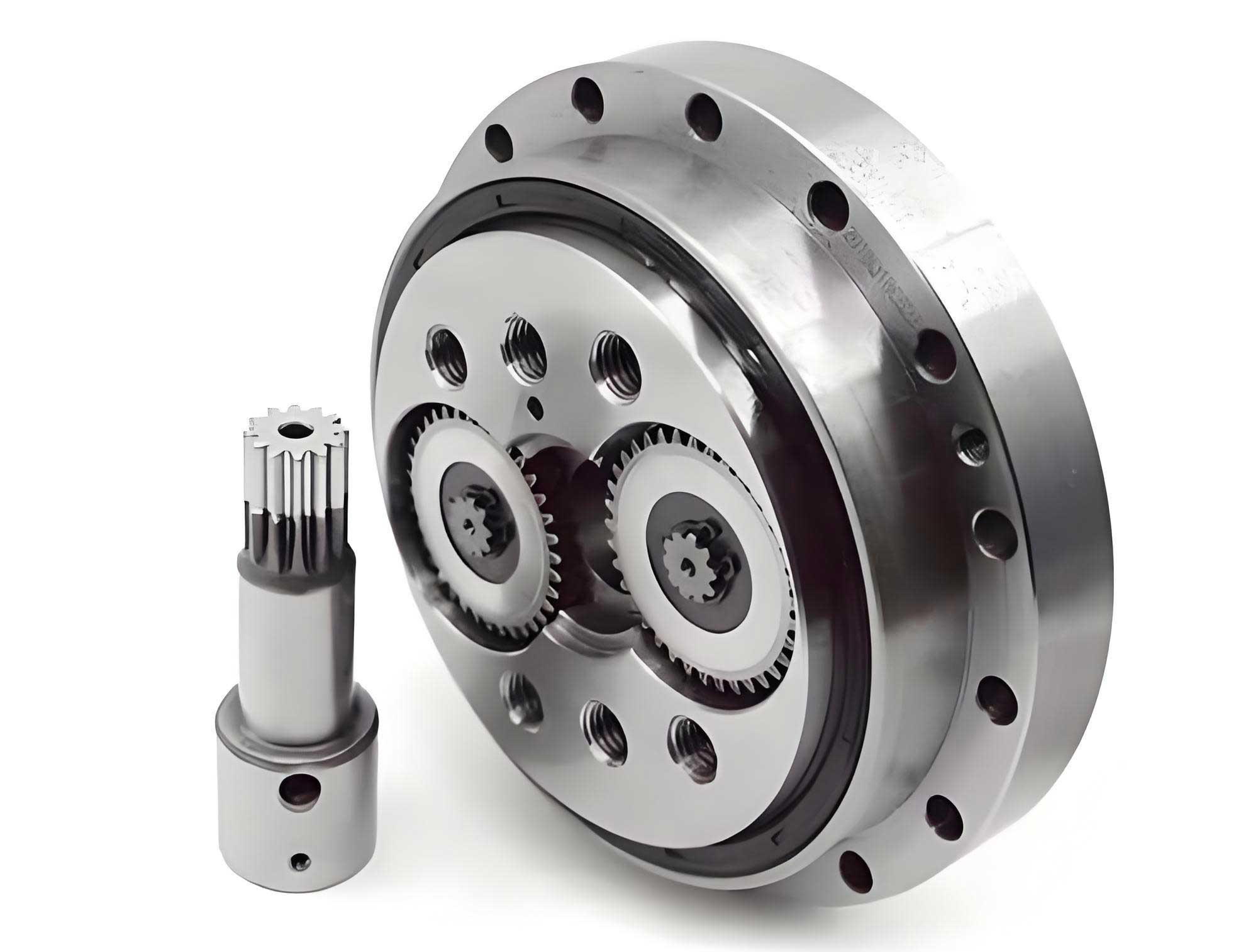
Vibration signals effectively reflect the health status of mechanical components and are widely used in fault diagnosis. In recent years, numerous studies have employed methods such as neural networks, deep learning, time-frequency analysis, and blind deconvolution for diagnosing the rotary vector reducer. While these approaches, particularly data-driven ones like deep learning, can achieve high diagnostic accuracy, they often require vast amounts of labeled training data covering various fault types. In contrast, signal processing methods based on time-domain, frequency-domain, or time-frequency domain analysis can accomplish fault diagnosis with relatively limited data. Nonetheless, existing signal processing methods are primarily effective for single-fault scenarios. In practice, faults such as cracks and pitting in the rotary vector reducer often occur simultaneously or sequentially due to lubrication issues, manufacturing errors, and improper loads. The signals collected by sensors are typically a coupled mixture from multiple fault sources, significantly complicating diagnosis. Consequently, precisely separating and extracting coupled fault features under conditions of composite faults, reciprocating motion, and time-varying speeds remains a critical challenge in the fault diagnosis of rotary vector reducers.
Blind Source Separation technology offers a promising solution, as it can recover multiple source signals from mixed observations without prior knowledge of the transmission channels. Among BSS techniques, Sparse Component Analysis is particularly suitable for mechanical fault diagnosis. Unlike Independent Component Analysis, which requires source signals to be statistically independent, SCA relies on the more readily satisfied assumption of sparsity. The SCA framework primarily involves two steps: estimating the mixing matrix and reconstructing the source signals. For mixing matrix estimation, clustering algorithms are preferred. The Density Peak Clustering algorithm shows potential for this task as it can identify cluster centers based on local density and relative distance without requiring prior knowledge of the number of clusters. For source signal reconstruction, Compressed Sensing algorithms, such as the Orthogonal Matching Pursuit algorithm, provide an efficient approach by solving an L1-norm optimization problem, avoiding the NP-hard nature of L0-norm minimization.
To address the aforementioned challenges, this study proposes a novel blind fault separation method for the rotary vector reducer under reciprocating motion and variable speed conditions. The method integrates Time-Frequency Ridge Extraction with an improved Sparse Component Analysis technique. The proposed framework first employs the Ridge Extraction from Time-Frequency images algorithm to synchronously截取vibration signals from constant-speed segments of the robotic arm’s operation. Subsequently, a combined盲源分离method termed SMF-DPC-OMP, which incorporates sinC-based Morphological Filtering, Density Peak Clustering, and Orthogonal Matching Pursuit, is applied to separate and extract the composite faults from the stationary signals.
Mathematical Model of Blind Separation
The blind source separation problem, considering noise, can be modeled within the SCA framework as follows:
$$X_{m \times t} = A_{m \times n}S_{n \times t} + V_{m \times t}$$
where \(X\) is the observation matrix (i.e., the collected vibration signals), \(A\) is the unknown mixing matrix, \(S\) represents the unknown source signals which are assumed to be sparse, \(V\) denotes additive noise or random interference, \(m\) is the number of sensors, \(n\) is the number of source signals, and \(t\) is the observation time in seconds. The objective is to estimate both \(A\) and \(S\) given only \(X\).
Ridge Extraction from Time-Frequency Images for Stationary Segment Isolation
Under variable speed conditions, such as the start-up, constant velocity, and deceleration phases of a robotic arm, the vibration signals from the rotary vector reducer are non-stationary. Direct application of fault diagnosis methods designed for stationary signals becomes ineffective. Therefore, isolating segments of data corresponding to constant speed operation is a crucial preprocessing step. Short-Time Fourier Transform is an effective tool for capturing time-varying frequency content. The STFT of a signal \(x(\tau)\) is defined as:
$$Q(t, f) = \int_{\mathbb{R}} x(\tau) h_{\sigma}(\tau – t) e^{-j 2\pi f \tau} d\tau$$
where \(h_{\sigma}(\tau – t)\) is a window function (e.g., a Gaussian window) centered at time \(t\), and \(Q(t, f)\) is the time-frequency representation. The instantaneous frequency can be estimated by extracting the ridge from the TFR, which corresponds to the path of maximum energy. The ridge \(D(t)\) is defined as:
$$D(t) = \arg \max_{f \in J} |Q(t, f)|, \quad t = t_0, \ldots, t_{N-1}$$
where \(J\) is the set of frequency bins. The proposed RETF algorithm iteratively identifies and tracks these ridges. The procedure is summarized in the following table:
| Step | Description |
|---|---|
| 1 | Initialize parameters and create a storage matrix \(K_i\). |
| 2 | Compute the STFT \(Q(t, f)\) of the time-domain signal \(x(t)\). |
| 3 | Find and mark the point of maximum energy \(\begin{bmatrix} t_0 \\ f_0 \end{bmatrix}\), storing it as the first column of \(K_i\). |
| 4 | Set \(Q(t_0, f)=0\) for \(f \in [f_0 – \Delta f, f_0 + \Delta f]\) to suppress the found ridge locally. |
| 5 | Find the next maximum energy point \(\begin{bmatrix} t’_0 \\ f’_0 \end{bmatrix}\) within a neighborhood defined by \(t_{\alpha} \in [t_0-1, t_0+1]\) and \(f_{\alpha} \in [f_0-F, f_0+F]\). |
| 6 | Store the new point in \(K_i\). |
| 7 | Suppress the region around the new point in \(Q(t, f)\). |
| 8 | Repeat steps 5-7 until a time or frequency boundary is reached, then return to step 1 for a new ridge/potential storage matrix. |
| 9 | Terminate the algorithm when the remaining energy in the TFR falls below a threshold \(\epsilon\). |
By analyzing the trajectory of the extracted ridges, different operational phases (acceleration, constant speed, deceleration) of the rotary vector reducer can be clearly distinguished. The constant-speed phase segments are then synchronously截取from the multi-sensor observation signals for subsequent analysis.
Blind Source Separation via SMF-DPC-OMP
The core of the proposed fault separation method lies in the SMF-DPC-OMP algorithm, which is applied to the截取stationary signals.
sinC-based Morphological Filtering for Signal Enhancement
Morphological filtering is a nonlinear signal processing technique effective for enhancing impulsive features. The core operations are dilation \(\oplus\), erosion \(\Theta\), opening \(\circ\), and closing \(\bullet\), defined for a discrete signal \(f(n)\) and a structuring element \(g(m)\) as:
$$(f \Theta g)(n) = \min_{m} [f(n+m) – g(m)]$$
$$(f \oplus g)(n) = \max_{m} [f(n-m) + g(m)]$$
$$(f \circ g)(n) = ((f \Theta g) \oplus g)(n)$$
$$(f \bullet g)(n) = ((f \oplus g) \Theta g)(n)$$
To suppress both positive and negative noise, the opening-closing (OC) and closing-opening (CO) filters are typically combined. An average combination filter is used to mitigate statistical bias:
$$y(n) = \frac{OC(f(n)) + CO(f(n))}{2}$$
The choice of the structuring element \(g\) is critical. This study proposes using the sinC function as a novel structuring element:
$$\text{sinC}(x) = \frac{\sin(\pi x)}{\pi x}$$
The sinC function, with its main lobe and decaying side lobes, is well-suited for matching and extracting transient冲击patterns commonly associated with gear faults in the rotary vector reducer. The parameters of the structuring element are its length \(L\) and main-lobe ratio \(p\). The SMF effectively enhances the signal’s信噪比and sparsity by突出impulsive components while suppressing noise, providing a cleaner signal for the subsequent clustering stage.
Mixing Matrix Estimation via Density Peak Clustering
After SMF enhancement, the filtered observation signals are used to estimate the mixing matrix \(A\). In the sparse domain (often achieved via a Short-Time Fourier Transform or simply using the frequency-domain representation), the columns of the source matrix \(S\) are assumed to be sparse. Under this condition, the observation vectors \(X(:, k)\) at each time-frequency point \(k\) lie close to the lines defined by the columns of the mixing matrix \(A\). Therefore, estimating \(A\) becomes a clustering problem of these observation vectors in the scatter plot.
The DPC algorithm is employed for this task. For a dataset \(U = \{u_1, u_2, …, u_R\}\), DPC operates based on two assumptions: cluster centers are surrounded by neighbors with lower local density, and they are at a relatively large distance from points with higher density. The algorithm involves calculating two quantities for each data point \(u_i\):
1. Local Density \(\rho_i\):
$$\rho_i = \sum_{j, j \neq i} \chi(d_{ij} – d_c)$$
where \(\chi(x)=1\) if \(x<0\) and \(0\) otherwise, \(d_{ij}\) is the distance between points \(i\) and \(j\), and \(d_c\) is a cutoff distance.
2. Minimum Distance to a Point of Higher Density \(\delta_i\):
$$\delta_i = \begin{cases}
\min_{j:\rho_j > \rho_i}(d_{ij}), & \text{if } \rho_i < \max(\rho) \\
\max_{j}(d_{ij}), & \text{if } \rho_i = \max(\rho)
\end{cases}$$
A decision graph is plotted with \(\rho\) and \(\delta\). Points with both high \(\rho\) and high \(\delta\) are selected as cluster centers. These cluster center vectors correspond to the estimated columns of the mixing matrix \(\hat{A}\) for the rotary vector reducer fault sources. This method does not require prior knowledge of the number of sources \(n\), as it can be inferred from the number of prominent cluster centers in the decision graph.
Source Signal Reconstruction via Orthogonal Matching Pursuit
With the estimated mixing matrix \(\hat{A}\), the final step is to reconstruct the source signals \(S\). This is formulated as a Compressed Sensing reconstruction problem. The observation model in the frequency domain can be written as:
$$Y = \Phi X$$
where \(Y\) is the vectorized frequency-domain observation, \(X\) is the vectorized sparse source matrix to be recovered, and \(\Phi\) is the sensing matrix constructed from \(\hat{A}\). Specifically, if \(\hat{A} = [a_1, a_2, …, a_n]\), and \(E\) is the Fourier basis matrix, the sensing matrix \(\Phi\) is built by expanding each column \(a_j\) with \(E\):
$$\Phi = \begin{bmatrix}
E \cdot a_{11} & E \cdot a_{12} & \cdots & E \cdot a_{1n} \\
E \cdot a_{21} & E \cdot a_{22} & \cdots & E \cdot a_{2n} \\
\vdots & \vdots & \ddots & \vdots \\
E \cdot a_{m1} & E \cdot a_{m2} & \cdots & E \cdot a_{mn}
\end{bmatrix}$$
The OMP algorithm is then used to solve for the sparse vector \(X\). OMP is a greedy iterative algorithm that selects the column of \(\Phi\) most correlated with the current residual in each iteration, then solves a least squares problem to update the signal estimate and residual. The steps are:
| Step | OMP Algorithm Procedure |
|---|---|
| 1 | Initialize residual \(r_0 = Y\), index set \(\Lambda_0 = \emptyset\), iteration counter \(\ell=0\). |
| 2 | Find the index \(\lambda_{\ell} = \arg \max_j |\langle r_{\ell}, \phi_j \rangle|\), where \(\phi_j\) is the j-th column of \(\Phi\). |
| 3 | Update the index set: \(\Lambda_{\ell} = \Lambda_{\ell-1} \cup \{\lambda_{\ell}\}\). |
| 4 | Solve the least squares problem: \(x_{\ell} = \arg \min_x \|Y – \Phi_{\Lambda_{\ell}} x\|_2\). |
| 5 | Update the residual: \(r_{\ell+1} = Y – \Phi_{\Lambda_{\ell}} x_{\ell}\). |
| 6 | Increment \(\ell\). If stopping criteria (e.g., sparsity level or residual norm) not met, go to Step 2. |
The reconstructed vector \(X\) is then reshaped and transformed back to the time domain via the inverse Fourier transform, yielding the separated source signals \(\hat{S}_1(t), \hat{S}_2(t), …, \hat{S}_n(t)\). A final Fast Fourier Transform is applied to each separated signal for spectral analysis and fault characteristic frequency identification related to the rotary vector reducer components.
Experimental Validation and Results
The proposed method was validated using vibration data collected from a test bench simulating the single-joint reciprocating motion of an agricultural robot arm equipped with a rotary vector reducer. Two accelerometers were mounted perpendicularly on the reducer’s housing. Composite faults involving simultaneous wear on the sun gear and a planetary gear were introduced into the rotary vector reducer. The arm performed reciprocating motions between 0° and 90° at a speed of 100°/s, creating non-stationary conditions. The key characteristic frequencies for the specific rotary vector reducer model (RV40E, reduction ratio 121) are calculated as follows:
| Component | Frequency Calculation | Description |
|---|---|---|
| Sun Gear Fault Frequency (\(f_s\)) | \(f_s = f_1 + f_3\) | \(f_1\): Sun gear rotation frequency, \(f_3\): Carrier (output) rotation frequency. |
| Planetary Gear Fault Frequency (\(f_p\)) | \(f_p = f_2 – f_3\) | \(f_2\): Planetary gear rotation frequency relative to fixed frame. |
| First Stage Mesh Frequency (\(f_{1c}\)) | \(f_{1c} = \frac{Z_1 Z_2 Z_4}{Z_1 + Z_2 Z_4} f_1\) | \(Z_1, Z_2, Z_4\): Teeth numbers of sun, planetary, and pin gears. |
For the test conditions, the theoretical fault frequencies were \(f_s \approx 38.34\) Hz and \(f_p \approx 10.83\) Hz.
The raw vibration signal from one sensor was first analyzed using STFT. The resulting time-frequency representation was highly blurred due to strong transient impacts and variable speed, making it difficult to visually distinguish operational phases. Applying the RETF algorithm successfully extracted clear ridges, from which the constant-speed phase (between approximately 0.35s and 0.70s) was accurately identified and截取for both sensor channels.
The截取stationary signals were then processed by the SMF-DPC-OMP algorithm. The SMF stage effectively enhanced the periodic冲击components. The DPC algorithm was applied to the frequency-domain representation of the filtered observations. The decision graph showed two distinct cluster centers, correctly indicating two underlying fault sources. These centers were used to construct the mixing matrix \(\hat{A}\). Finally, the OMP algorithm reconstructed the source signals in the frequency domain.
The Fourier spectra of the two separated signals were analyzed. One spectrum showed prominent spectral lines at 37.5 Hz and its harmonics, closely matching the theoretical sun gear fault frequency (\(f_s\)). The other spectrum showed dominant lines at 10.94 Hz and its harmonics, aligning with the theoretical planetary gear fault frequency (\(f_p\)). The results demonstrated that the proposed RETF-SMF-DPC-OMP method successfully separated the composite fault features of the rotary vector reducer, which were heavily coupled in the original observed spectra.
A comparative analysis was performed against a traditional method combining standard morphological filtering with SCA (MF-SCA). The results indicated that while the MF-SCA method could not fully separate the composite faults (both separated spectra contained mixed frequencies from both faults), the proposed method achieved complete separation. Furthermore, the SMF-DPC-OMP algorithm required approximately 75% less computational time than the MF-SCA method, and produced cleaner spectra with fewer interference components and sidebands, facilitating easier and more reliable fault identification for the rotary vector reducer.
Conclusion
This study presented a novel blind fault separation methodology for diagnosing composite faults in rotary vector reducers operating under realistic, non-stationary conditions such as reciprocating motion and variable speeds. The integration of Time-Frequency Ridge Extraction with an improved Sparse Component Analysis framework addresses key challenges in this domain. The RETF algorithm provides a robust tool for identifying and isolating constant-speed operational segments from complex time-frequency representations, which is a critical preprocessing step for applying stationary signal analysis techniques. The proposed SMF-DPC-OMP algorithm forms the core of the blind separation process. The sinC-based morphological filter effectively enhances the sparse, impulsive nature of fault signatures in the rotary vector reducer. The Density Peak Clustering algorithm reliably estimates the number of fault sources and the mixing matrix without prior knowledge. Finally, the Orthogonal Matching Pursuit algorithm enables efficient and accurate reconstruction of the source signals in the frequency domain.
Experimental results from a rotary vector reducer test bench with simultaneous sun gear and planetary gear wear faults confirmed the efficacy of the proposed method. It successfully separated the coupled fault features, with the extracted characteristic frequencies closely matching theoretical values. The advantages over existing methods include superior separation performance, significant reduction in computational time, and the generation of cleaner, more interpretable spectra. This work provides a practical and effective reference for the fault feature extraction of rotary vector reducers in agricultural robots and other industrial applications. Future work will focus on extending this approach to underdetermined scenarios (where sensors are fewer than sources) and exploring its application to acoustic-based fault diagnosis of rotating machinery.