
Abstract
The straight bevel gear transmission system serves as a core component in locomotive power systems, and its operational characteristics directly influence the safety and reliability of train operations. To investigate the nonlinear vibration behaviors of straight bevel gear pairs and eliminate chaotic motion, this thesis proposes an intelligent chaos control strategy based on a fuzzy neural network integrated with an improved particle swarm optimization algorithm. A seven-degree-of-freedom nonlinear dynamic model of the straight bevel gear transmission system is established by considering time-varying meshing stiffness, tooth side clearance, comprehensive transmission errors, and damping effects. The governing differential equations are derived using Newton’s second law, followed by nondimensionalization and reduction to state-space form. Numerical solutions are obtained via the fourth-fifth order Runge-Kutta method, and bifurcation diagrams, phase portraits, and Poincaré sections are utilized to analyze the dynamic behavior under varying parameters including the time-varying meshing stiffness coefficient, comprehensive transmission error coefficient, load coefficient, and meshing frequency ratio. A five-layer fuzzy neural network chaos controller is designed with inputs derived from the distances between adjacent points on the Poincaré surface. To overcome the limitations of standard particle swarm optimization, including premature convergence and poor local search capability, several improvements are proposed: Piecewise chaotic mapping for population initialization, nonlinear adaptive inertia weights, adaptive learning factors, and an adaptive Lévy flight mechanism based on dynamic centroid migration. The improved algorithm is validated using eight benchmark functions, demonstrating superior convergence accuracy and global search performance. The optimized fuzzy neural network controller is then applied to realize chaos control of the straight bevel gear transmission system. Numerical simulation results indicate that chaotic motion, quasi-periodic motion, and multi-periodic motion can be effectively suppressed and stabilized onto target periodic orbits, including period-one, period-two, period-three, and period-four motions, thereby providing a theoretical reference for enhancing the operational stability and reliability of locomotive gear transmission systems.
Keywords: straight bevel gear, nonlinear dynamics, chaos control, fuzzy neural network, improved particle swarm optimization
1 Introduction
1.1 Research Background and Significance
The straight bevel gear transmission is a quintessential mechanical power transmission component widely deployed in locomotive traction systems. Within the HXD1D electric locomotive used on the Lanzhou-Xinjiang railway, straight bevel gear pairs are integrated into the traction motor reduction device to achieve a 90-degree power redirection between the motor output shaft and the wheel axle. The primary advantages of straight bevel gears include high load-carrying capacity, smooth transmission, large transmission ratios, high efficiency, and structural compactness. However, the operational environment of locomotive gear systems involves high torque, frequent start-stop cycles, and complex load conditions, which collectively give rise to highly intricate dynamic characteristics.
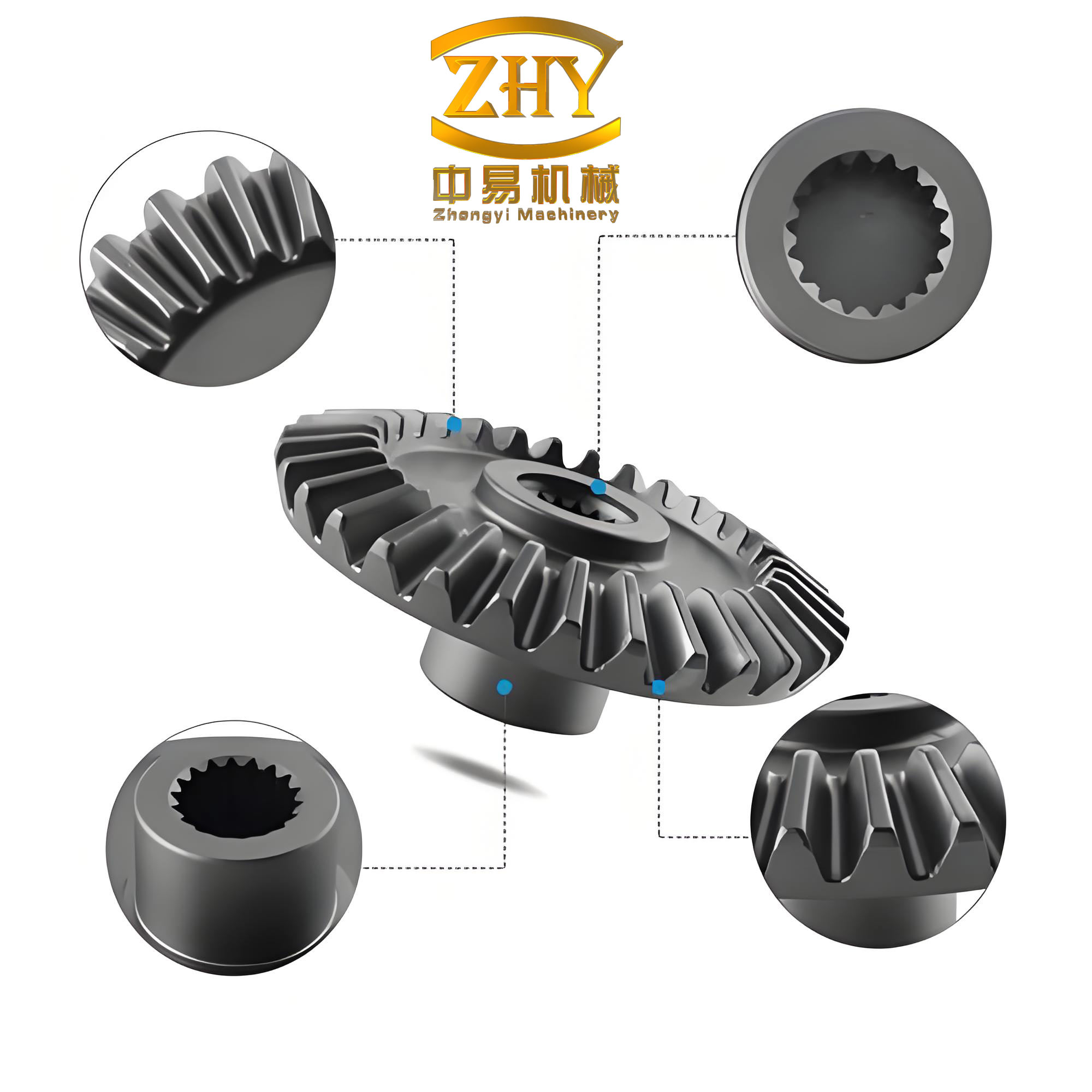
During actual operation, the straight bevel gear transmission system is subjected to two categories of excitation: external excitations from prime mover torque fluctuations and load reaction torques, and internal excitations including time-varying meshing stiffness, tooth profile transmission errors, and mesh-in/mesh-out impacts. These nonlinear factors, together with tooth backlash and friction, are mutually coupled and introduce abundant nonlinear dynamic phenomena such as jump phenomena, bifurcations, and chaos. Chaotic motion, in particular, manifests as irregular oscillations that can severely degrade the performance of the gear transmission system, shorten equipment service life, and threaten the high-speed stability of locomotives. Traditional linear analysis methods are no longer adequate for precisely predicting the behavior of high-performance gear systems. Therefore, a thorough nonlinear vibration analysis and effective chaos suppression for straight bevel gear transmission systems are of significant engineering importance.
1.2 Literature Review
1.2.1 Dynamics of Bevel Gear Systems
Extensive research has been devoted to the nonlinear dynamics of bevel gear systems. Wang Sanmin and colleagues investigated a seven-degree-of-freedom spiral bevel gear transmission system and obtained torsional, lateral, and axial vibration displacements and velocities under various operating conditions. Their findings demonstrated that as the meshing frequency varies, the system enters chaos through period-doubling bifurcations, while variations in support stiffness induce quasi-periodic bifurcations leading to chaotic vibrations. Wang Lihua studied spiral bevel gear systems and observed that as the meshing frequency changes, the system exhibits multiple steady-state responses including single-period harmonic responses, multi-period subharmonic responses, quasi-periodic responses, and chaotic responses. Qiu Huansong incorporated the influence of lubricating oil films and analyzed how changes in clearance affect nonlinear characteristics of gear systems. Wang Shilong established a multi-degree-of-freedom nonlinear dynamic model of spiral bevel gears considering time-varying friction forces and friction coefficients. Feng Gang explored cracked bevel gear transmission systems and concluded that cracks significantly affect vibration responses and increase the likelihood of quasi-periodic and chaotic phenomena. Zhao Ning studied an eight-degree-of-freedom straight bevel gear transmission system under partial nonlinear factors and identified geometric transmission errors as the dominant factor affecting gear vibration when manufacturing errors are neglected.
1.2.2 Chaos Control of Gear Transmission Systems
Chaos control approaches can be broadly categorized into feedback and non-feedback methods. Feedback methods, such as the OGY method and continuous feedback control, offer advantages of not requiring explicit model information and possessing good trajectory tracking capability; however, they demand relatively accurate mathematical models and well-defined target functions. Non-feedback methods, which introduce small external perturbations such as signals, constant biases, or weak parameter modulations, are simpler in design and implementation but provide no assurance of control stability.
Liu Xiaoning applied the OGY method to control chaos in a single-stage gear system with backlash nonlinearity. Chen Xuesen extended this work by incorporating time-varying meshing stiffness. Tian Yaping implemented an improved OGY algorithm for chaos control of a high-dimensional non-smooth gear transmission system. Wang Jingyue employed three non-feedback methods to stabilize chaotic motion of a single-stage gear system to periodic motion. Ghasem developed a nonlinear time-varying dynamic model of a spur gear pair incorporating backlash, time-varying stiffness, static transmission errors, and external excitation, and devised sliding mode and adaptive sliding mode control laws to suppress chaotic vibrations. Farshidianfar used Melnikov analysis to predict chaos in spur gear pairs and applied additional control excitation to eliminate chaos. For multi-degree-of-freedom systems, Liu Xiaoning considered a three-degree-of-freedom gear model and continuously drove system states onto local stable manifolds of periodic orbits. Li Yinong applied fuzzy controllers and fuzzy PID controllers for chaos control of three-degree-of-freedom gear transmission systems. Gao Yang utilized a simplified radial basis function neural network controller for the same class of systems.
With deeper investigations into gear transmission dynamics, it has become increasingly evident that the complexity of chaotic systems often makes their analytical models arduous to establish precisely. Consequently, intelligent control methods, including fuzzy logic and neural network control, which rely on input-output data rather than exact mathematical models, are gaining popularity as a research hotspot for chaos control in gear systems. The application of such data-driven intelligent control strategies to the straight bevel gear transmission system, however, remains relatively underexplored, necessitating further investigation into the underlying control mechanisms.
1.2.3 Fuzzy Neural Networks
Fuzzy neural networks synergistically combine the linguistic interpretability of fuzzy logic with the adaptive learning capability of neural networks. Unlike conventional neural networks’ “black-box” behavior, fuzzy neural networks provide a logical framework through IF-THEN rule bases, enabling satisfactory modeling of complex nonlinear relationships. Sun Zengqi proposed a fuzzy neural network based on the Takagi-Sugeno model, where the network nodes and parameters can be initialized applying qualitative system knowledge, and learning algorithms enable fast convergence to the desired input-output relation. Wang Xuewu highlighted that fuzzy neural networks benefit from both fuzzy logic’s uncertain information processing and neural networks’ self-learning capability. Liu Ding employed a radial basis function neural network approach for chaos control without requiring an analytical model of the chaotic system. Wang Xin completed fuzzy neural network applications in gear thermal analysis by training the network with samples under single-parameter variations and subsequently calculating heat generation trends under multi-parameter variations. Lu Wenjuan proposed an adaptive control method based on fuzzy neural networks and realized simulation of adaptive fuzzy control for manipulators. Lin Da applied sliding mode control and fuzzy neural adaptive control to achieve control and synchronization of uncertain or unknown chaotic systems. Li Xiuying developed a T-S fuzzy neural network controller optimized by particle swarm optimization, demonstrating good control performance. Li Jiejia optimized fuzzy RBF neural networks with PSO for furnace temperature control. Xi Meng proposed a self-organizing fuzzy neural network with hybrid learning algorithms for nonlinear system modeling. Recent advances in fuzzy neural network design have considerably broadened the applicability of intelligent control strategies to complex engineering systems.
1.2.4 Particle Swarm Optimization
Particle swarm optimization, originally proposed by Kennedy and Eberhart, is a population-based global optimization algorithm inspired by the foraging behavior of bird flocks. While PSO is structurally simple and easy to implement, its global search capability is frequently impeded by premature convergence and susceptibility to local optima, particularly when addressing high-dimensional complex objective functions. Numerous improvements have been proposed in the literature. Kuang Fangjun combined Tent chaotic mapping with artificial bee colony advantages to enhance cooperative evolution in PSO. Wang Hao introduced global neighborhood search strategies and global-best particle perturbation mechanisms. Fan Chengli proposed a particle swarm algorithm with convergence factors to address high-dimensional complex multimodal functions. Yang Jingming improved multi-objective PSO to enhance convergence and diversity. Qian Xiaoyu developed opposition-based learning competitive PSO incorporating local search. More recently, Qiu proposed a game-theoretic strategy update mechanism to improve PSO performance. These collective efforts underscore the potential of PSO as a powerful metaheuristic tool when appropriately modified to match the problem structure.
1.3 Main Research Content of This Thesis
The primary objective of this thesis is to establish a faithful dynamic model of a straight bevel gear transmission system and to realize effective chaos suppression via a hybrid intelligent control strategy. The main research contents are organized as follows:
Chapter 1 introduces the research background, significance, and state-of-the-art in gear dynamics, chaos control, fuzzy neural networks, and particle swarm optimization.
Chapter 2 establishes a seven-degree-of-freedom nonlinear dynamic model of the straight bevel gear system considering tooth clearance, time-varying meshing stiffness, comprehensive transmission errors, damping, and load. After deriving nondimensionalized state equations, the Runge-Kutta method is adopted to solve the system under various parameters. Bifurcation diagrams and phase portraits are constructed to analyze the impacts of time-varying meshing stiffness, comprehensive transmission error, meshing frequency, and load on the system dynamic behavior.
Chapter 3 elaborates on the design of a fuzzy neural network chaos controller, including a technical roadmap and system control flow diagram. The standard PSO is presented, and several enhancements are introduced: Piecewise chaotic mapping initialization, adaptive learning factors, nonlinear adaptive inertia weights, and an adaptive Lévy flight mechanism based on dynamic centroid migration. The improved algorithm (IPSO) is validated against multiple benchmark functions.
Chapter 4 presents numerical control simulations of the straight bevel gear transmission system, where the IPSO-optimized fuzzy neural network controller is applied to chaos, quasi-periodic, and multi-periodic motion states, stabilizing them onto desired periodic orbits.
2 Bifurcation Analysis of the Straight Bevel Gear Transmission System
2.1 Dynamic Excitation Mechanisms
The dynamic behavior of the straight bevel gear transmission system is governed by several excitation sources whose accurate mathematical description is of paramount importance for the fidelity of the dynamic model.
2.1.1 Time-Varying Meshing Stiffness
The meshing stiffness of a gear pair refers to the capacity to resist elastic deformation during the meshing process. As the contact ratio of gear pairs typically lies between 1 and 2, alternation between single-tooth-pair and double-tooth-pair contact zones causes periodic variation in the comprehensive meshing stiffness. In this thesis, the straight bevel gear meshing stiffness is expressed as:
$$k_h(t) = k_m + \sum_{l=1}^{N} k_{kl} \cos(l\Omega_h t + \phi_{kl})$$
where $k_m$ is the mean meshing stiffness, $k_{kl}$ is the $l$-th order harmonic amplitude, $\Omega_h$ is the meshing frequency, and $\phi_{kl}$ is the phase angle. For computational precision and practical relevance, only the first-order term is retained, yielding:
$$k_h(\tau) = k_m + k_{k1} \cos(\Omega \tau + \phi_{k1})$$
where $\tau = \Omega_n t$ is the nondimensionalized time, and $\Omega = \Omega_h/\Omega_n$ is the meshing frequency ratio.
2.1.2 Comprehensive Transmission Error
Deviations between the actual and theoretical angular displacements due to manufacturing imperfections, installation errors, and elastic deformations constitute the gear transmission error, which significantly impacts vibration, noise, and transmission precision. The comprehensive transmission error is modeled as:
$$e_n(t) = \sum_{l=1}^{N} A_l \cos(l\Omega_h t + \phi_l)$$
where $A_l$ is the $l$-th harmonic amplitude, and $\phi_l$ represents the initial phase. In the nondimensionalized formulation, the comprehensive transmission error is represented by the coefficient $f_e = A_{el}/b_h$.
2.1.3 Tooth Side Clearance
Tooth side clearance is the minimum static gap measured along the line of action between the driving tooth flank and the driven tooth non-working flank. It serves essential roles in preventing tooth jamming due to thermal expansion, reducing meshing impacts and noise, providing space for lubricating oil films, and accommodating manufacturing tolerances. To express its influence on the dynamics, a piecewise clearance function is employed:
$$f(\lambda, b_n) = \begin{cases} \lambda – b_n, & \lambda > b_n \\ 0, & |\lambda| \leq b_n \\ \lambda + b_n, & \lambda < -b_n \end{cases}$$
where $\lambda$ is the relative torsional displacement along the meshing line, and $b_n$ is half of the tooth side clearance. This function characterizes three distinct meshing states: contact on the driving flank, separation, and contact on the reverse flank.
2.1.4 Meshing Damping
The meshing damping represents the energy dissipation capability of the gear pair during engagement. It is typically expressed as:
$$c_h = 2\mu \sqrt{k_m m_e}$$
where $m_e$ is the equivalent mass, $\mu$ is the damping coefficient (typically 0.03–0.17 for straight bevel gears), and $k_m$ is the average meshing stiffness.
2.2 Establishment of the Seven-Degree-of-Freedom Dynamic Model
The primary geometric parameters of the straight bevel gear pair studied in this thesis are summarized in Table 1.
| Parameter | Symbol | Driving Gear | Driven Gear |
|---|---|---|---|
| Number of teeth | $z_1$, $z_2$ | 47 | 53 |
| Module (mm) | $m$ | 2 | |
| Normal pressure angle (°) | $\alpha_n$ | 20 | |
| Pitch cone angle (°) | $\delta_1$, $\delta_2$ | 41.57 | 48.43 |
| Cone distance (mm) | $R$ | 70.8 | 70.8 |
| Tip angle (°) | $\theta_{a1}$, $\theta_{a2}$ | 2.35 | 1.95 |
| Tip cone angle (°) | $\delta_{a1}$, $\delta_{a2}$ | 43.92 | 50.34 |
| Root angle (°) | $\theta_{f1}$, $\theta_{f2}$ | 1.95 | 2.35 |
| Root cone angle (°) | $\delta_{f1}$, $\delta_{f2}$ | 39.62 | 46.04 |
| Gear ratio | $u$ | 1.13 | |
| Addendum modification coefficient | $x_1$, $x_2$ | 0.04 | -0.04 |
| Addendum (mm) | $h_{a1}$, $h_{a2}$ | 2.08 | 1.92 |
| Tooth height (mm) | $h$ | 4.5 | |
| Dedendum (mm) | $h_{f1}$, $h_{f2}$ | 2.42 | 2.58 |
| Pitch diameter (mm) | $d_1$, $d_2$ | 94 | 106 |
Employing the lumped mass method and considering only the translational vibrations along the coordinate axes and torsional vibrations about the respective gear axes, the seven-degree-of-freedom dynamic model of the straight bevel gear system is established. The generalized coordinates are $\{X_1, Y_1, Z_1, \theta_1, X_2, Y_2, Z_2, \theta_2\}$, where subscripts 1 and 2 denote the driving and driven gears respectively, $X_i$, $Y_i$, $Z_i$ represent translational displacements, and $\theta_i$ represents torsional angular displacements. By applying Newton’s second law, the governing differential equations are derived as:
$$I_1 \ddot{\theta}_1 + r_1 F_t = T_1$$
$$I_2 \ddot{\theta}_2 + r_2 F_t = -T_2$$
$$m_j \ddot{y}_j + c_{yj} \dot{y}_j + k_{yj} y_j = F_{yj}$$
$$m_j \ddot{z}_j + c_{zj} \dot{z}_j + k_{zj} z_j = F_{zj}$$
$$m_j \ddot{x}_j + c_{xj} \dot{x}_j + k_{xj} x_j = F_{xj}$$
where $m_j$ and $I_j$ are the mass and moment of inertia of gear $j$, $k_{ij}$ and $c_{ij}$ ($i=x, y, z$; $j=1, 2$) are the support stiffness and damping coefficients, and $F_t$, $F_{xj}$, $F_{yj}$, $F_{zj}$ are the dynamic meshing force components.
The relative displacement of the gear pair along the meshing line, denoted by $\lambda$, is expressed as:
$$\lambda = X_1 – X_2 + a_1(Y_1 – Y_2) + a_2(Z_1 – Z_2) + r_1\theta_1 – r_2\theta_2 – e_n(t)$$
where $a_1 = \cos\delta_1 \sin\alpha_n$, $a_2 = \cos\delta_1 \cos\alpha_n$, and $r_1$, $r_2$ are the base circle radii of the two gears.
The dynamic meshing force and its components are given by:
$$F_n = k_h(t) f(\lambda, b_n) + c_h \dot{\lambda}$$
$$F_x = F_n(\cos\delta_1 \sin\alpha_n + \sin\delta_1 \cos\alpha_n)$$
$$F_y = F_n(\sin\delta_1 \sin\alpha_n – \cos\delta_1 \cos\alpha_n)$$
$$F_z = F_n \cos\alpha_n$$
By introducing the relative torsional displacement $\lambda$ as a new degree of freedom to eliminate the torsional vibrations $\theta_1$ and $\theta_2$, and then performing nondimensionalization, the dimensionless governing equations of the straight bevel gear system are obtained. The detailed nondimensionalized formulation is:
$$\begin{aligned} \ddot{x}_1 + 2\xi_{x1} \dot{x}_1 + k_{x1} x_1 + a_1 k_{h1} f(x_{13}) + a_1 c_{h1} \dot{x}_{13} &= 0 \\ \ddot{y}_1 + 2\xi_{y1} \dot{y}_1 + k_{y1} y_1 – a_2 k_{h1} f(x_{13}) – a_2 c_{h1} \dot{x}_{13} &= 0 \\ \ddot{z}_1 + 2\xi_{z1} \dot{z}_1 + k_{z1} z_1 – a_3 k_{h1} f(x_{13}) – a_3 c_{h1} \dot{x}_{13} &= 0 \\ \ddot{x}_2 + 2\xi_{x2} \dot{x}_2 + k_{x2} x_2 + a_1 k_{h2} f(x_{13}) + a_1 c_{h2} \dot{x}_{13} &= 0 \\ \ddot{y}_2 + 2\xi_{y2} \dot{y}_2 + k_{y2} y_2 – a_2 k_{h2} f(x_{13}) – a_2 c_{h2} \dot{x}_{13} &= 0 \\ \ddot{z}_2 + 2\xi_{z2} \dot{z}_2 + k_{z2} z_2 – a_3 k_{h2} f(x_{13}) – a_3 c_{h2} \dot{x}_{13} &= 0 \\ \ddot{x}_{13} + a_1 \ddot{x}_1 + a_2 \ddot{z}_1 – a_1 \ddot{x}_2 – a_2 \ddot{z}_2 + \ddot{x}_{13} &= f_{pm} + f_{pv} \cos(\Omega \tau) \end{aligned}$$
where $x_j = X_j/b_h$, $y_j = Y_j/b_h$, $z_j = Z_j/b_h$ are the dimensionless coordinates, $b_h$ is the standard tooth clearance, $\Omega_{ij} = (k_{ij}/m_j)^{1/2}$, $k_{ij} = (\Omega_j/\Omega_n)^2$, $\xi_j = c_j/(2m_j\Omega_n)$, $\Omega_n = (k_m/m_e)^{1/2}$, and $m_e = I_1 I_2/(r_1^2 I_2 + r_2^2 I_1)$.
For numerical computation, the dimensionless equations are reduced to a set of first-order state equations of dimension 14, represented compactly as $\dot{\mathbf{x}} = \mathbf{f}(\mathbf{x}, \tau)$, where the state vector is $\mathbf{x} = [x_1, \dot{x}_1, x_2, \dot{x}_2, \ldots, x_{13}, \dot{x}_{13}]^T$. The full state equations are provided below:
$$x_1′ = x_2$$
$$x_2′ = -k_{x1} x_1 – 2\xi_{x1} x_2 – a_1 k_{h1} f(x_{13}) – a_1 c_{h1} x_{14}$$
$$x_3′ = x_4$$
$$x_4′ = -k_{y1} x_3 – 2\xi_{y1} x_4 + a_2 k_{h1} f(x_{13}) + a_2 c_{h1} x_{14}$$
$$x_5′ = x_6$$
$$x_6′ = -k_{z1} x_5 – 2\xi_{z1} x_6 + a_3 k_{h1} f(x_{13}) + a_3 c_{h1} x_{14}$$
$$x_7′ = x_8$$
$$x_8′ = -k_{x2} x_7 – 2\xi_{x2} x_8 – a_1 k_{h2} f(x_{13}) – a_1 c_{h2} x_{14}$$
$$x_9′ = x_{10}$$
$$x_{10}’ = -k_{y2} x_9 – 2\xi_{y2} x_{10} + a_2 k_{h2} f(x_{13}) + a_2 c_{h2} x_{14}$$
$$x_{11}’ = x_{12}$$
$$x_{12}’ = -k_{z2} x_{11} – 2\xi_{z2} x_{12} + a_3 k_{h2} f(x_{13}) + a_3 c_{h2} x_{14}$$
$$x_{13}’ = x_{14}$$
$$x_{14}’ = -c_1 x_2 – c_2 x_6 + c_1 x_8 + c_2 x_{12} – c_6 k_h f(x_{13}) – c_6 c_h x_{14} + f_{pm} + f_{pv} \cos(\Omega \tau)$$
where $c_1 = \cos\delta_1 \sin\alpha_n$, $c_2 = \cos\delta_1 \cos\alpha_n$, $c_3 = \cos\alpha_n$, $c_4 = \sin\alpha_n$, $c_5 = \cos\alpha_n$, $c_6 = \cos\alpha_n$, and primes denote differentiation with respect to the nondimensional time $\tau$.
2.3 Numerical Analysis Tools
To characterize the dynamic responses of the straight bevel gear transmission system, several standard nonlinear dynamics diagnostic tools are employed:
(1) Bifurcation diagrams: These diagrams depict changes in the system’s steady-state behavior as a control parameter is varied continuously. The horizontal axis represents the control parameter, while the vertical axis represents a characteristic state variable sampled at the excitation period. Period-doubling routes, tangent bifurcations, and transitions to chaos can be readily identified.
(2) Phase portraits: Trajectories in the displacement-velocity plane reveal qualitative aspects of the system motion. Closed curves indicate periodic motion, dense trajectory bands with folded structures suggest chaos, and closed loops forming toroidal structures correspond to quasi-periodic motion.
(3) Poincaré sections: By sampling the system state at intervals of the excitation period, continuous trajectories are mapped to discrete points. Periodic motions appear as a finite number of isolated points, quasi-periodic motions appear as closed curves, and chaotic motions appear as collections of irregularly scattered points.
2.4 Effect of System Parameters on Bifurcation Behavior
The system parameters utilized in numerical simulations are set as follows unless otherwise stated: $k_{x1}=k_{y1}=k_{z1}=k_{x2}=k_{y2}=k_{z2}=1.25$, $\xi_{x1}=\xi_{y1}=\xi_{z1}=\xi_{x2}=\xi_{y2}=\xi_{z2}=0.42$, $f_e=0.2$, $\Omega=1$, $f_{pm}=0.05$, $f_{pv}=0$, $b=1$, $k_{h1}=k_{h2}=0.5$, $\xi_h=0.06$, $\xi_{h1}=\xi_{h2}=0.012$, and $k_h=1+a\cos(\Omega\tau)$.
2.4.1 Influence of the Time-Varying Meshing Stiffness Coefficient $a$
Taking the time-varying meshing stiffness coefficient $a$ as the bifurcation parameter, the bifurcation diagram in the range $a \in [0.1, 1.00]$ is displayed in Figure 2.6 of the original research. As $a$ increases from 0 toward 1, the system traverses a rich sequence of dynamic states: chaotic motion initially, followed by a transition to period-3 motion, then period-doubling bifurcations from period-3 to period-6, further period-doubling to period-12 and period-24, transition to quasi-periodic motion, and finally recurrence of chaotic motion. The key findings are summarized in Table 2.
| Parameter range | Dynamic state | Poincaré mapping |
|---|---|---|
| $a \in [0.1, 0.35)$ | Chaotic motion | Non-periodic scattered points |
| $a \in (0.35, 0.4)$ | Period-3 motion | 3 discrete points |
| $a \in (0.4, 0.427)$ | Period-6 motion | 6 discrete points |
| $a \in (0.427, 0.437)$ | Period-12 motion | 12 discrete points |
| $a \in (0.437, 0.441)$ | Period-24 motion | 24 discrete points |
| $a \in (0.441, 0.451)$ | Quasi-periodic motion | Closed curve on section |
| $a > 0.451$ | Chaotic motion | Non-periodic scattered points |
2.4.2 Influence of the Comprehensive Transmission Error Coefficient $f_e$
With $a=0.25$, the comprehensive transmission error coefficient $f_e$ is varied across the range $[0, 2.00]$. The evolution of the dynamic behavior exhibits remarkable complexity. For $f_e < 0.1048$, the system executes stable single-period motion. At $f_e = 0.1048$, a bifurcation jump leads to period-2 motion, followed by period-4 and period-8 motions through successive period-doubling bifurcations. At $f_e = 0.149$, Hopf bifurcation occurs, and the system transitions into chaotic motion, which persists until $f_e = 0.2315$, where the system emerges into a period-3 window. Period-doubling then produces period-6 and period-12 motions, followed by a return to chaos. Another bifurcation at $f_e = 0.378$ marks the onset of period-6 motion, which subsequently undergoes reverse period-doubling to period-3. Between $f_e=0.973$ and $f_e=1.015$, chaos reappears. Further increases in $f_e$ lead to quasi-periodic motion at $f_e=1.067$ and period-4 motion at $f_e=1.072$. At higher values, reverse period-doubling from period-8 to period-4 to period-2 occurs, culminating in single-period motion at $f_e=1.467$. A comprehensive summary is presented in Table 3.
| Parameter range | Dynamic state |
|---|---|
| $f_e \in [0, 0.1048)$ | Period-1 motion |
| $f_e = 0.1048$ | Bifurcation jump to period-2 |
| $f_e \in (0.1048, 0.133)$ | Period-2 motion |
| $f_e = 0.133$ | Period-4 motion |
| $f_e = 0.143$ | Period-8 motion |
| $f_e = 0.149$ | Hopf bifurcation |
| $f_e \in (0.15, 0.2315)$ | Chaotic motion |
| $f_e = 0.2315$ | Period-3 motion |
| $f_e = 0.2379$ | Period-6 motion |
| $f_e = 0.243$ | Period-12 motion |
| $f_e \in (0.243, 0.378)$ | Chaotic motion |
| $f_e = 0.378$ | Jump to period-6 |
| $f_e \in (0.972, 1.015)$ | Chaotic motion with embedded periodic windows |
| $f_e = 1.067$ | Quasi-periodic motion |
| $f_e = 1.072$ | Period-4 motion |
| $f_e = 1.089$ | Period-8 motion |
| $f_e = 1.096$ | Period-4 motion |
| $f_e = 1.103$ | Period-2 motion |
| $f_e = 1.467$ | Period-1 motion |
2.4.3 Influence of the Load Coefficient $f_{pm}$
Setting $a=0.25$ and varying the load coefficient $f_{pm}$ over $[0, 1.00]$, the system response exhibits the patterns shown in Table 4.
| Parameter range | Dynamic state |
|---|---|
| $f_{pm} \in [0, 0.00151)$ | Period-1 motion |
| $f_{pm} \in (0.00151, 0.00248)$ | Period-2 motion |
| $f_{pm} \in (0.00248, 0.04001)$ | Chaotic motion |
| $f_{pm} \in (0.04023, 0.041)$ | Quasi-periodic motion |
| $f_{pm} = 0.041$ | Multi-period motion |
| $f_{pm} \in (0.041, 0.0432)$ | Period-6 motion, then period-3 |
| $f_{pm} \in (0.048, 0.0663)$ | Chaotic motion |
| $f_{pm} = 0.0673$ | Period-12 motion |
| $f_{pm} = 0.07$ | Period-8 motion |
| $f_{pm} = 0.075$ | Period-4 motion |
| $f_{pm} = 0.084$ | Period-2 motion |
| $f_{pm} = 0.09$ | Period-1 motion |
2.4.4 Influence of the Meshing Frequency Ratio $\Omega$
With $a=0.25$, the meshing frequency ratio $\Omega$ is swept over $[0.50, 2.00]$. The system exhibits period-1 motion until $\Omega \approx 0.65$, followed by period-2 motion, and period-4 motion near $\Omega=0.83$. Further increases lead to period-8 and multi-periodic motions, with chaotic motion appearing in the interval $\Omega \in (0.843, 1.033)$. Within this chaotic region, a period-3 window exists near $\Omega=1.066$, followed by period-6 motion at $\Omega=1.099$ and multi-periodic states. Between $\Omega=1.249$ and $\Omega=1.253$, the system transitions from quasi-periodic to period-8 to period-4 motion. As $\Omega$ approaches 1.3, the system settles into stable single-period motion. The detailed observations are listed in Table 5.
| Parameter range | Dynamic state |
|---|---|
| $\Omega = 0.56$ | Period-1 motion |
| $\Omega = 0.65$ | Period-2 motion |
| $\Omega = 0.74$ | Period-2 motion (changed trajectory) |
| $\Omega = 0.83$ | Period-4 motion |
| $\Omega = 0.833$ | Period-8 motion |
| $\Omega = 0.839$ | Multi-period motion |
| $\Omega \in (0.843, 1.033)$ | Chaotic motion with period-3 window |
| $\Omega = 1.033$ | Chaotic motion |
| $\Omega = 1.066$ | Period-3 motion |
| $\Omega = 1.099$ | Period-6 motion |
| $\Omega \in (1.117, 1.249)$ | Multi-period motion |
| $\Omega = 1.249$ | Quasi-periodic motion |
| $\Omega = 1.251$ | Period-8 motion |
| $\Omega = 1.253$ | Period-4 motion |
| $\Omega = 1.255$ | Period-4 motion |
| $\Omega = 1.257$ | Period-8 motion |
| $\Omega = 1.28$ | Period-2 motion |
| $\Omega = 1.3$ | Period-1 motion |
These comprehensive bifurcation analyses establish a complete map of dynamic states for the straight bevel gear transmission system. They provide the fundamental basis for selecting appropriate control parameters and target orbits in the subsequent chaos control studies.
3 Design of the IPSO-Based Fuzzy Neural Network Chaos Controller
3.1 Architecture of the Fuzzy Neural Network Controller
The fuzzy neural network controller designed in this thesis adopts a five-layer structure, which includes the input layer, fuzzification layer, fuzzy rule layer, defuzzification layer, and output layer.
Input layer: The controller inputs are chosen based on the Poincaré section distance information. Specifically, the inputs are $d(k) = \|X(k) – X(k-1)\|$ and $d(k-1) = \|X(k-1) – X(k-2)\|$, where $X(k)$ represents the coordinate of the system state at the $k$-th iteration on the Poincaré section.
Fuzzification layer: Each input is partitioned into five fuzzy subsets, denoted as $\mu_i^m$, which correspond to linguistic labels: very large, large, medium, small, and very small. The membership functions are Gaussian-type and are expressed as:
$$\mu_i^m = \exp\left(-\frac{\|D_i – C_{im}\|^2}{b_{im}}\right)$$
where $i = 1, 2$ denotes the input index, $m = 1, 2, \ldots, 5$ denotes the fuzzy subset index, $C_{im}$ is the center of the $m$-th membership function associated with the $i$-th input, and $b_{im}$ is the corresponding width parameter.
Fuzzy rule layer: Each node in this layer represents a fuzzy rule. The output of each rule node is computed by the multiplication of the incoming membership degrees:
$$\alpha_i = \mu_1^m \cdot \mu_2^m$$
where $\alpha_i$ ($i = 1, 2, \ldots, 25$) denotes the firing strength of the $i$-th fuzzy rule.
Defuzzification layer: The firing strengths are normalized as follows:
$$\bar{\alpha}_i = \frac{\alpha_i}{\sum_{j=1}^{M} \alpha_j}$$
where $M = 25$ is the total number of fuzzy rules.
Output layer: The controller output, i.e., the perturbation quantity $U(k)$, is calculated as:
$$U(k) = \sum_{i=1}^{M} \bar{\alpha}_i w_i = \mathbf{\bar{\alpha}}^T \mathbf{w}$$
where $\mathbf{w} = [w_1, w_2, \ldots, w_M]^T$ is the weight matrix connecting the defuzzification layer to the output layer. The output is constrained to satisfy $-u_{max} \leq U(k) \leq u_{max}$, where $u_{max}$ is the maximum allowable perturbation.
3.2 Chaos Control Strategy and Technical Roadmap
The overall control strategy employs the fuzzy neural network controller to generate a small perturbation $\Delta\Omega$ applied to the meshing frequency ratio of the straight bevel gear system. When the system has been iterated for 200 times while still exhibiting chaotic motion, the controller is activated to initiate the perturbation.
The system control flowchart proceeds as follows: the state vector $X(k)$ is sampled at each iteration, and the distance $d(k)$ is computed. The controller receives the historical distances $[d(k), d(k-1)]$ as inputs and generates the perturbation $U(k)$ based on the fuzzy inference and neural network weights. The perturbed system parameter becomes $\Omega = \Omega_0 + U(k)$, where $\Omega_0$ denotes the nominal value corresponding to the chaotic state. The control objective is to drive the system onto a target periodic orbit, characterized by a desired value $d^*$ of the distance on the Poincaré section.
The fitness function used in the particle swarm optimization is constructed based on the cumulative deviation between the actual Poincaré distance and the desired distance:
$$f(P_i) = \sum_{k=1}^{L} \left| d(k) – d^* \right| = \sum_{k=1}^{L} \left| \|X(k) – X(k-1)\| – d^* \right|$$
where $L$ is the data sequence length. A smaller fitness value indicates that the controller parameters encoded by particle $P_i$ lead to a system response closer to the target periodic orbit.
3.3 Improved Particle Swarm Optimization Algorithm
3.3.1 Standard Particle Swarm Optimization
In the canonical PSO, each particle $i$ is characterized by its position vector $P_i = [p_{i1}, p_{i2}, \ldots, p_{is}]$ and velocity vector $v_i = [v_{i1}, v_{i2}, \ldots, v_{is}]$ in an $s$-dimensional search space. During the iterative process, each particle updates its velocity and position by tracking its personal best position $p_{pbest}$ and the global best position $p_{gbest}$:
$$v_{is}(t+1) = w v_{is}(t) + c_1 R_1 (p_{pbest,s} – p_{is}(t)) + c_2 R_2 (p_{gbest,s} – p_{is}(t))$$
$$p_{is}(t+1) = p_{is}(t) + v_{is}(t+1)$$
where $w$ is the inertia weight, $c_1$ and $c_2$ are the learning factors, and $R_1$, $R_2$ are uniform random numbers in $[0, 1]$.
3.3.2 Chaotic Initialization Using Piecewise Mapping
To enhance the initial diversity of the particle swarm and enable uniform coverage of the solution space, a Piecewise chaotic map is adopted for population initialization:
$$p(t+1) = \begin{cases} \frac{p(t)}{q}, & 0 \leq p(t) < q \\ \frac{p(t) – q}{0.5 – q}, & q \leq p(t) < 0.5 \\ \frac{1 – q – p(t)}{0.5 – q}, & 0.5 \leq p(t) < 1 – q \\ \frac{1 – p(t)}{q}, & 1 – q \leq p(t) < 1 \end{cases}$$
where $q = 1$ is a control parameter. The chaotic sequence exhibits ergodicity and non-repetition properties, thereby mitigating the spatial clustering caused by random initialization and reducing the probability of premature convergence.
3.3.3 Adaptive Learning Factors
To balance global exploration in the early stages and local exploitation in the later stages, the learning factors $c_1$ and $c_2$ are designed as nonlinear time-varying functions:
$$c_1(t) = 2 \sin\left(\frac{\pi}{2}\left(1 – \frac{t}{T}\right)\right)$$
$$c_2(t) = 2 \sin\left(\frac{\pi}{2}\cdot\frac{t}{T}\right)$$
where $t$ denotes the current iteration number and $T$ is the maximum number of iterations. In the early stage, $c_1 > c_2$ emphasizes individual cognition, allowing particles to search extensively; in the later stage, $c_1 < c_2$ strengthens social learning and accelerates convergence toward the global optimum.
3.3.4 Adaptive Inertia Weight
A nonlinear time-varying inertia weight is formulated as:
$$w(t) = w_{Max} – (w_{Max} – w_{Min}) \cdot \tan\left(0.875 \left(1 – \left(\frac{t}{T}\right)^k\right)\right)$$
where $w_{Max} = 0.9$, $w_{Min} = 0.1$, and $k = 0.6$ are empirical control parameters. This schedule maintains a relatively large weight at the beginning for comprehensive global exploration and gradually reduces it to enable refined local searches around the promising regions.
3.3.5 Lévy Flight Strategy Based on Dynamic Centroid Migration
Lévy flight is a random walk model characterized by heavy-tailed step-size distributions, which enables occasional long jumps that help particles escape from local optima. The Lévy distributed random step size is computed as:
$$s = \frac{\mu}{|v|^{1/\beta}}$$
where $\mu \sim N(0, \sigma_\mu^2)$, $v \sim N(0, \sigma_v^2)$, $\sigma_v = 1$, $\beta = 1.5$, and
$$\sigma_\mu = \left[\frac{\Gamma(1+\beta)\sin(\pi\beta/2)}{\Gamma((1+\beta)/2)\cdot 2^{(\beta-1)/2}\beta}\right]^{1/\beta}$$
In this thesis, an adaptive Lévy flight improvement mechanism based on dynamic centroid migration is proposed. Instead of using the individual worst solution as the reference point, the global best solution $p_{gbest}$ is utilized to establish a heterogeneous step-size search model:
$$p_{is}(t+1) = b_2 p_{is}(t) + b_1 p_{gbest,s} + 0.01 \cdot s \cdot (p_{gbest,s} – p_{is}(t))$$
where the weighting coefficients are defined as:
$$b_1 = \frac{t}{T}, \quad b_2 = 1 – \frac{t}{T}$$
At the beginning of iterations ($t \to 0$), $b_2 > b_1$, allowing the search to prioritize diversity. As iterations proceed, the weighting shifts progressively toward the global best solution, and when $t = T$, $b_2 \to 0$, the algorithm concentrates entirely on fine-grained search near $p_{gbest}$.
3.3.6 Dynamic Selection Mechanism
To coordinate the synergistic effects of the Lévy flight strategy with the adaptive parameters ($w$, $c_1$, and $c_2$), a Bernoulli-distribution-based dynamic selection mechanism is designed. In each iteration, with probability $p = 0.5$, particles update their positions using the canonical velocity-position update formula; otherwise, they employ the Lévy flight position update. The selection rule is:
$$p_{is}(t+1) = \begin{cases} p_{is}(t) + v_{is}(t+1), & \text{if } A < 0.5 \\ b_2 p_{is}(t) + b_1 p_{gbest,s} + 0.01 s (p_{gbest,s} – p_{is}(t)), & \text{if } A \geq 0.5 \end{cases}$$
where $A$ is a uniform random number in $[0, 1]$.
3.4 Validation of the Improved Particle Swarm Optimization
To evaluate the performance of the improved PSO (IPSO), eight benchmark functions with distinct characteristics are utilized: Ackley, Alpine, Eggholder, Griewank, Levy, Rastrigin, Schaffer, and Weierstrass functions. The mathematical expressions, search ranges, and theoretical optima are summarized in Table 6.
| Function | Expression | Range | Optimum |
|---|---|---|---|
| Griewank | $f(x) = \frac{1}{4000}\sum_{i=1}^{N} x_i^2 – \prod_{i=1}^{N} \cos\left(\frac{x_i}{\sqrt{i}}\right) + 1$ | $[-600, 600]^N$ | 0 |
| Rastrigin | $f(x) = \sum_{i=1}^{N} [x_i^2 – 10\cos(2\pi x_i) + 10]$ | $[-5.12, 5.12]^N$ | 0 |
| Ackley | $f(x) = -a\exp\left(-b\sqrt{\frac{1}{N}\sum_{i=1}^N x_i^2}\right) – \exp\left(\frac{1}{N}\sum_{i=1}^N \cos(c x_i)\right) + a + e$ | $[-32, 32]^N$ | 0 |
| Schaffer | $f(x) = 0.5 + \frac{\sin^2\left(\sqrt{\sum_{i=1}^N x_i^2}\right) – 0.5}{\left(1 + 0.001\sum_{i=1}^N x_i^2\right)^2}$ | $[-100, 100]^N$ | -1 |
| Alpine | $f(x) = \sum_{i=1}^N |x_i \sin(x_i) + 0.1 x_i|$ | $[-10, 10]^N$ | 0 |
| Eggholder | $f(x, y) = \sum_{i=1}^N \left[-(y_i+47)\sin\sqrt{|y_i + \frac{x_i}{2} + 47|} – x_i \sin\sqrt{|x_i – (y_i+47)|}\right]$ | $[-512, 512]^N$ | -959.6407 |
| Levy | $f(x) = \sum_{i=1}^{N-1} (x_i – 1)^2 (1 + \sin^2(3\pi x_{i+1})) + \sin^2(3\pi x_1) + (x_N – 1)^2 (1 + \sin^2(2\pi x_N))$ | $[-10, 10]^N$ | 0 |
| Weierstrass | $f(x) = \sum_{i=1}^N \sum_{k=0}^{20} 0.5^k \cos(2\pi 3^k (x_i + 0.5)) – N \sum_{k=0}^{20} 0.5^k \cos(\pi 3^k)$ | $[-0.5, 0.5]^N$ | 0 |
The algorithm parameters are set as: population size $N = 150$, maximum number of iterations $T = 1500$, and dimension $dim = 20$. The comparative optimization results between the standard PSO and the improved PSO are presented in Table 7.
| Function | Standard PSO | Improved PSO |
|---|---|---|
| Ackley | 5.0574e-04 | 8.8817e-16 |
| Alpine | 0.145319 | 6.0014e-141 |
| Eggholder | 7.9501e+02 | 9.5964e+02 |
| Griewank | 1.1504e-07 | 0 |
| Levy | 0.090218 | 3.0395e-07 |
| Rastrigin | 8.188847 | 0 |
| Schaffer | -0.995116 | -1 |
| Weierstrass | 2.503866 | 0 |
The results clearly demonstrate that the improved PSO achieves significantly better optimization accuracy on all benchmark functions, frequently reaching the theoretical global optimum. The enhancements successfully mitigate premature convergence and improve the global search capability, making the IPSO well-suited for optimizing the fuzzy neural network controller parameters in the straight bevel gear chaos control problem.
4 Control Simulation of the Straight Bevel Gear System
4.1 Parameter Settings and Control Objectives
The system parameters employed in the control simulations are identical to those used in the bifurcation analysis. The fuzzy neural network controller parameters are optimized using the improved PSO with a population size of 150 and a maximum of 100 iterations. The parameter search ranges are set as $\omega \in [-3, 3]$, $b \in [-3, 3]$, and $c \in [-3, 3]$. The control perturbation is activated after the system has undergone 200 iterations in the uncontrolled chaotic state.
4.2 Control of Chaotic Motion to Periodic Orbits
4.2.1 Control to Period-One Motion
Setting the initial frequency ratio $\Omega = 0.862$, the straight bevel gear system operates in a chaotic state. The phase portrait exhibits a tangled, folded trajectory, and the Poincaré section displays non-periodically scattered points. After activating the fuzzy neural network controller, the system reaches a stable period-one orbit within a short time. The corresponding Poincaré section contains exactly one point. The perturbation quantity output from the controller rapidly converges from a time-varying value to a constant value, with the system becoming stable after approximately 13 iterations of disturbance. The optimized controller parameters achieving this period-one control are listed in Table 8.
| $w$ | $b_{1m}$ and $b_{2m}$ | $C_{1m}$ and $C_{2m}$ |
|---|---|---|
| -1.7350 | -1.5721, -1.2846 | -1.6693, -1.7799 |
| -0.1285 | -1.6599, -1.3353 | -0.8814, -0.6160 |
| -1.7931 | -0.9319, -0.3782 | -0.9916, -1.2283 |
| -0.2182 | -1.2521, -0.7416 | -0.6149, -1.1715 |
| -0.3479 | -1.5100, -0.5805 | -0.1482, 0.6168 |
4.2.2 Control to Period-Two Motion
Under identical system conditions, the fuzzy neural network controller is optimized with a different target orbit. After activation, the chaotic motion of the straight bevel gear system is stabilized onto a period-two orbit, verified by the appearance of exactly two points on the Poincaré section. The system reaches this state after only 4 perturbation iterations. The controller parameters are summarized in Table 9.
| $w$ | $b_{1m}$ and $b_{2m}$ | $C_{1m}$ and $C_{2m}$ |
|---|---|---|
| -0.0803 | -1.4886, 0.9841 | 0.1473, 0.1163 |
| 0.4621 | -0.4757, 0.0399 | 0.2704, 1.0648 |
| 0.3427 | 1.6503, -0.1176 | -0.6700, -1.2135 |
| 0.0148 | -0.8108, 0.2946 | -0.4539, -1.0073 |
| -0.5040 | 0.4740, 0.0034 | -0.1899, -0.1414 |
4.2.3 Control to Period-Four Motion
With the same initial chaotic state at $\Omega = 0.862$, the controller is further optimized to drive the straight bevel gear system onto a period-four orbit. The Poincaré section exhibits exactly four discrete points, confirming successful period-four control. The system achieves stability after approximately 10 perturbation iterations. The corresponding controller parameters are provided in Table 10.
| $w$ | $b_{1m}$ and $b_{2m}$ | $C_{1m}$ and $C_{2m}$ |
|---|---|---|
| -0.3808 | -1.9091, -2.4368 | -1.3317, -3.0000 |
| -0.8313 | -0.5714, -2.1608 | -3.0000, -2.4170 |
| -2.6842 | -1.0141, -0.2008 | -2.2337, -1.6978 |
| -1.0908 | -2.7536, -0.0543 | -1.9870, -1.5736 |
| -1.0023 | -1.4612, -1.0337 | -2.0165, -2.5512 |
4.3 Control of Multi-Periodic Motion
The control capability of the proposed strategy extends beyond chaotic motion to multi-periodic motion states. Using the same system parameters but an initial frequency ratio $\Omega = 1.23$, the straight bevel gear system is initially in a multi-periodic state. The IPSO-optimized fuzzy neural network controller successfully stabilizes the system onto a period-four orbit. The perturbation applied is small in magnitude and rapidly converges to a constant value, achieving period-four motion after 6 perturbation iterations. The controller parameters are listed in Table 11.
| $w$ | $b_{1m}$ and $b_{2m}$ | $C_{1m}$ and $C_{2m}$ |
|---|---|---|
| -0.1367 | -2.1635, -2.3862 | -0.4952, -2.5571 |
| -0.1795 | -2.5761, -0.1598 | 0.4362, 2.0490 |
| -1.9758 | -2.6333, -0.3840 | 0.0898, -2.0714 |
| 0.6067 | -0.0083, -1.9657 | -2.6324, -2.2060 |
| 0.1060 | -0.3019, -0.1404 | -2.0047, -1.0362 |
For the initial frequency ratio $\Omega = 1.256$, where the straight bevel gear system exhibits multi-periodic motion, two distinct control tasks are accomplished. The first task drives the system to a period-two orbit, achieving stabilized periodic motion after 5 perturbation iterations. The second task drives the same initial state to a period-one orbit, requiring 17 perturbation iterations. These results demonstrate the flexibility of the fuzzy neural network controller in steering the straight bevel gear system to arbitrarily specified target periodic orbits. The optimized parameters for period-two control are given in Table 12, and those for period-one control are given in Table 13.
| $w$ | $b_{1m}$ and $b_{2m}$ | $C_{1m}$ and $C_{2m}$ |
|---|---|---|
| 0.8521 | -0.6408, 0.0869 | 0.7505, 0.5505 |
| 1.1088 | 0.0077, -0.6882 | 1.2175, 1.0331 |
| -0.2776 | -1.0447, -0.8659 | 1.2129, -1.6556 |
| 0.2193 | -0.0434, -1.0045 | 0.6876, 0.3119 |
| -0.7776 | 0.2196, -0.2264 | 0.7880, 0.2864 |
| $w$ | $b_{1m}$ and $b_{2m}$ | $C_{1m}$ and $C_{2m}$ |
|---|---|---|
| -0.0860 | -0.2337, -0.2914 | -0.3830, 0.0324 |
| 0.2936 | -0.2419, -0.2212 | -0.2916, -0.9098 |
| 0.0336 | 0.1427, -0.0342 | -0.1172, -0.2678 |
| -0.0086 | -0.1308, -0.1198 | 0.0809, 0.0434 |
| -0.0457 | -0.1515, -0.0812 | -0.1964, -0.2044 |
4.4 Control with the Load Coefficient as the Perturbation Parameter
In this set of simulations, the load coefficient $f_{pm}$ is chosen as the perturbation parameter instead of the meshing frequency ratio. The system parameters are adjusted as follows: $k_{x1}=k_{y1}=k_{z1}=k_{x2}=k_{y2}=k_{z2}=1.25$, $\xi_{x1}=\xi_{y1}=\xi_{z1}=\xi_{x2}=\xi_{y2}=\xi_{z2}=0.05$, $f_e=0.025$, $\Omega=1$, $f_{pv}=0$, $b=1$, $k_{h1}=k_{h2}=0.25$, $\xi_h=0.13$, $\xi_{h1}=\xi_{h2}=0.19$, and $a=0.15$.
With an initial load coefficient $f_{pm} = 0.002$, the straight bevel gear system exhibits chaotic motion. The IPSO-optimized fuzzy neural network controller is activated after 200 iterations, and the system is successfully stabilized onto a period-two orbit within approximately 20 perturbation iterations. The Poincaré section of the controlled system shows exactly two points, validating the period-two control. The optimized controller parameters are listed in Table 14.
| $w$ | $b_{1m}$ and $b_{2m}$ | $C_{1m}$ and $C_{2m}$ |
|---|---|---|
| -0.0860 | -0.2337, -0.2914 | -0.3830, 0.0324 |
| 0.2936 | -0.2419, -0.2212 | -0.2916, -0.9098 |
| 0.0336 | 0.1427, -0.0342 | -0.1172, -0.2678 |
| -0.0086 | -0.1308, -0.1198 | 0.0809, 0.0434 |
| -0.0457 | -0.1515, -0.0812 | -0.1964, -0.2044 |
When the initial load coefficient is set to $f_{pm} = 0.016$, the straight bevel gear system operates in a quasi-periodic state, characterized by a closed-loop distribution on the Poincaré section. Applying the IPSO-optimized fuzzy neural network controller, the quasi-periodic motion is effectively suppressed, and the system converges to a period-two orbit within 5 perturbation iterations. The small and rapidly stabilizing perturbation confirms the effectiveness of the proposed control scheme in handling quasi-periodic dynamics of the straight bevel gear transmission system.
5 Conclusion and Outlook
5.1 Conclusion
This thesis has comprehensively investigated the nonlinear dynamics and chaos control of a straight bevel gear transmission system used in locomotive gearboxes. The primary contributions and conclusions are summarized as follows:
(1) Establishment and analysis of the nonlinear dynamic model. A seven-degree-of-freedom nonlinear dynamic model of the straight bevel gear transmission system was established using the lumped mass method, incorporating time-varying meshing stiffness, tooth side clearance, comprehensive transmission errors, damping, and external loads. Through nondimensionalization and numerical integration using the fourth-fifth order Runge-Kutta method, the bifurcation characteristics were systematically analyzed. The results revealed that the straight bevel gear system exhibits abundant nonlinear phenomena when system parameters vary, including single-period, multi-period (period-2, period-3, period-4, period-6, period-8, period-12), quasi-periodic, and chaotic motions. The transition routes include period-doubling bifurcations, Hopf bifurcations, and inverse period-doubling bifurcations. Specific chaotic parameter regions were identified for the time-varying meshing stiffness coefficient, comprehensive transmission error coefficient, load coefficient, and meshing frequency ratio, providing guidelines for parameter selection during system design and operation.
(2) Development of the improved particle swarm optimization algorithm. To overcome the limitations of the standard PSO, including premature convergence and insufficient local search accuracy, several enhancements were proposed. Piecewise chaotic mapping was adopted for population initialization to improve solution space coverage. Nonlinear adaptive inertia weights and adaptive learning factors were designed to balance global exploration and local exploitation. An adaptive Lévy flight mechanism based on dynamic centroid migration was introduced to enhance particle diversity and escape from local optima. A Bernoulli-distribution-based dynamic selection mechanism was established to coordinate the Lévy flight strategy with the adaptive parameters. Benchmark function tests demonstrated that the improved algorithm achieves significantly higher convergence accuracy and more robust global optimization performance compared to the standard PSO.
(3) Design and validation of the IPSO-FNN chaos controller. A five-layer fuzzy neural network controller was designed with inputs based on Poincaré section distances and output representing the perturbation quantity. The improved PSO was employed to optimize the controller parameters (weights, membership function centers, and widths). Numerical simulation results demonstrated that the proposed IPSO-FNN control strategy effectively stabilizes chaotic motion, quasi-periodic motion, and multi-periodic motion of the straight bevel gear transmission system onto target periodic orbits, including period-one, period-two, and period-four motions. The control perturbations are small in magnitude and converge rapidly to constant values, indicating high control efficiency and practical feasibility. The control strategy can be applied with either the meshing frequency ratio or the load coefficient as the perturbation parameter, offering flexibility in practical implementations.
5.2 Outlook
Several limitations of the present study suggest directions for future investigation:
(1) Model refinement. The dynamic model of the straight bevel gear transmission system in this thesis considered a subset of nonlinear factors. Future research should incorporate additional nonlinear elements such as thermo-elastohydrodynamic lubrication coupling, tooth surface friction variations, crack propagation, and wear degradation to enhance the fidelity of the model and improve the practical applicability of the theoretical results.
(2) Experimental validation. Due to limitations in experimental equipment and hardware conditions, the numerical simulation results have not been verified by experimental data. Future work should design bench-scale test setups with vibration response measurement, torque monitoring, and acoustic emission sensing to validate the theoretical predictions and control strategies in real-world scenarios.
(3) Controller enhancements. The computational efficiency of the IPSO-FNN controller could be further improved by incorporating online adaptation mechanisms, such as recursive least squares or extended Kalman filtering for real-time weight updates. Additionally, robustness analysis under parameter uncertainties and external disturbances would strengthen the practical viability of the proposed chaos control strategy for the straight bevel gear system.
(4) Multi-objective optimization. Future studies could explore multi-objective optimization frameworks that simultaneously minimize vibration amplitude, control effort, and energy consumption, offering a more comprehensive solution for the engineering control of straight bevel gear transmission systems.
In conclusion, this thesis has made significant strides toward understanding the complex nonlinear dynamics of the straight bevel gear transmission system and has proposed an effective intelligent chaos control approach based on a synergistically optimized fuzzy neural network. The findings provide a valuable theoretical foundation for vibration suppression, fault prevention, and reliability enhancement of high-performance gear transmission systems in locomotive applications.