
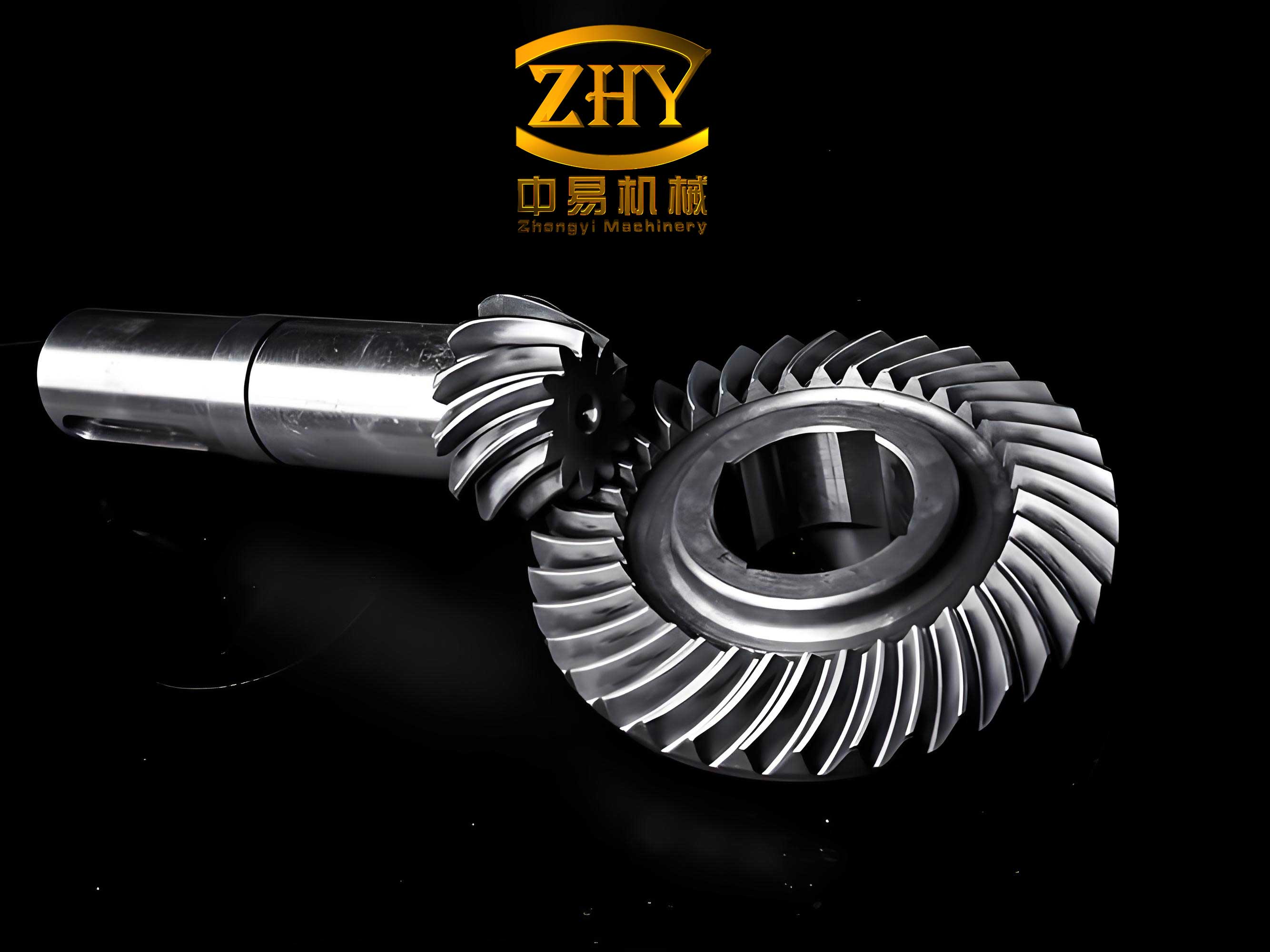
In my extensive work with power transmission systems, I have consistently found spiral bevel gears to be among the most fascinating and critical components. These gears are designed to transmit motion and power between intersecting axes, typically at a 90-degree angle. Compared to their straight bevel gear counterparts, spiral bevel gears offer a host of superior performance characteristics. Their primary advantages stem from the curved, helical shape of their teeth. This design leads to a larger contact ratio, meaning multiple teeth are in contact at any given moment during mesh. Consequently, this results in significantly higher load-carrying capacity, improved transmission efficiency, and remarkably smooth and quiet operation. The helical teeth also make the gear pair less sensitive to assembly errors and minor misalignments. Due to these exceptional properties, spiral bevel gears have become indispensable in high-performance and precision-demanding industries such as aerospace, marine propulsion, automotive differentials, and advanced machine tools. However, the very complexity that grants them superior performance also presents formidable challenges. Their intricate geometry, dynamic meshing behavior, sophisticated manufacturing processes involving complex machine settings and cutter geometry, coupled with the influences of load-induced deformations and assembly variations, make controlling their ultimate quality, durability, and noise-vibration-harshness (NVH) performance exceptionally difficult. Mastering spiral bevel gear technology represents a significant technical pinnacle in gear manufacturing. In this article, I will detail my methodology, grounded in solid geometrical theory and implemented through modern digital tools, for the precise three-dimensional modeling and subsequent finite element analysis of spiral bevel gears.
The foundational element of a spiral bevel gear’s tooth profile is the spherical involute. Understanding its generation is crucial for accurate modeling. Unlike cylindrical gears where the involute lies on a plane, the tooth profile of a bevel gear must lie on a sphere centered at the cone apex, as the tooth width tapers towards the apex. The spherical involute can be visualized as follows. Consider a base cone with its apex at point O and a base cone angle $\delta_b$. Now, imagine a generating plane, which is a circular disc of radius $R_b$ (the cone distance) also passing through O. As this generating plane rolls without slipping around the base cone, any point D on the disc traces a three-dimensional curve on the surface of a sphere with radius $R_b$—this curve is the spherical involute. To derive its mathematical model, I establish a right-handed Cartesian coordinate system with the origin at the cone apex O and the Z-axis aligned with the gear’s axis of rotation.
Let $R_b$ be the outer cone distance. Let $\delta_b$ be the base cone angle. Let $w$ be the variable cone angle for a point on the curve, measured from the Z-axis, ranging from the root cone angle $\delta_f$ to the face cone angle $\delta_a$. The generation process defines two key angular parameters: the roll angle of the base cone ($\beta$) and the roll angle of the generating plane ($\theta$). The relationship between these angles and the cone angle $w$ is governed by spherical trigonometry. For an arbitrary point D on the spherical involute, its Cartesian coordinates $(x, y, z)$ are given by the following set of equations, which I have extensively used and verified in my modeling work:
$$ x = R_b \cdot \sin(w) \cdot \cos(\sigma) $$
$$ y = R_b \cdot \sin(w) \cdot \cos(\sigma) $$
$$ z = R_b \cdot \cos(w) $$
In these equations, the parameter $\sigma$ is the azimuthal angle on the sphere and is itself a function of $w$ and $\delta_b$:
$$ \sigma = \frac{\arccos\left(\frac{\cos(w)}{\cos(\delta_b)}\right)}{\sin(\delta_b)} – \arccos\left(\frac{\tan(\delta_b)}{\tan(w)}\right) $$
This equation set fully defines the path of the spherical involute curve in space. The parameter $w$ serves as the primary variable, moving from the inner to the outer part of the tooth. The correct definition of $\sigma$ is critical, as it ensures the curve satisfies the condition of pure rolling between the generating plane and the base cone.
While the spherical involute defines the tooth profile shape in the profile direction, the spiral of a spiral bevel gear defines its lengthwise curvature. This spiral is typically a circular arc or a logarithmic curve when projected onto the pitch cone’s surface. For modeling a constant-tooth-depth design with a circular arc spiral, I often model the corresponding cutter path on the base cone, known as the base cone helix. Imagine a point P starting at the outer edge E of the base cone. As point P moves along a straight line towards the apex (i.e., the cone distance decreases from $R_b$ to an inner value $R_{bi}$), it also rotates around the Z-axis by an angle $\theta$. The trajectory of point P1, the final position, lies on the surface of the base cone and represents the base cone helix. Its parametric equations are simpler than those of the spherical involute:
$$ x = R_{bi} \cdot \sin(\delta_b) \cdot \cos(\theta) $$
$$ y = R_{bi} \cdot \sin(\delta_b) \cdot \sin(\theta) $$
$$ z = R_{bi} \cdot \cos(\delta_b) $$
Here, $R_{bi}$ is the instantaneous cone distance, varying linearly from the outer cone distance to the inner cone distance, and $\theta$ is the corresponding rotation angle, proportional to the linear travel and defined by the desired spiral angle $\beta_m$ at the mean cone distance.
| Parameter | Symbol | Pinion (Gear 1) | Gear (Gear 2) | Units |
|---|---|---|---|---|
| Module (at Large End) | $m$ | 5 | 5 | mm |
| Number of Teeth | $z$ | 20 | 40 | – |
| Pressure Angle | $\alpha$ | 20 | 20 | deg |
| Mean Spiral Angle | $\beta_m$ | 35 | 35 | deg |
| Hand of Spiral | – | Left | Right | – |
| Face Width | $b$ | 30 | 30 | mm |
With the mathematical foundation established, the practical task of creating a three-dimensional digital model begins. I prefer using parametric CAD software for this purpose, as it allows for design iteration and integration with analysis tools. However, a significant challenge arises because most mainstream CAD systems do not natively support the direct input of complex parametric equations like those for a spherical involute. To overcome this, I employ a computational workflow that bridges numerical computing and CAD modeling.
The first step is to compute discrete coordinate points along the spherical involute curve with high precision. For this, I utilize mathematical software like MATLAB. Its powerful matrix and array operations are ideal for this vectorized calculation. I define the gear parameters and the range for the variable $w$. For example, to get points from the root to the tip of the tooth:
$$ w = \delta_f + t \cdot (\delta_a – \delta_f) $$
where $t$ is a vector from 0 to 1, e.g., `t = linspace(0, 1, 100)`. I then compute the arrays for $x$, $y$, and $z$ using the equations (1) and (2). This generates a dense, ordered set of points that accurately represents the curve. The coordinates are then exported to a structured text file or, more conveniently, an Excel spreadsheet with columns for X, Y, and Z. The same process is repeated for the base cone helix or other guiding curves. This method ensures the mathematical integrity of the core geometry is preserved in the digital model.
Next, I import these coordinate files into the CAD environment, such as Autodesk Inventor. Here, I use the “Spline through Points” command to reconstruct a smooth curve through the imported point cloud. This effectively creates an exact digital representation of the spherical involute. To define one flank of a tooth, I need two spherical involutes: one for the convex (drive) side and one for the concave (coast) side. The second involute is generated by mirroring or by recalculating with a sign change and an offset corresponding to the tooth thickness angle. These two profile curves are then connected at their ends by circular arcs representing the tip land and the root fillet, forming a closed loop sketch on a conceptual spherical surface. I create such profile sketches at several cross-sections along the face width, typically at the heel (outer end), toe (inner end), and midpoint.
| Symbol | Description | Defining Equation/Relation |
|---|---|---|
| $R_b$ | Outer Cone Distance (Pitch Radius at Heel) | $R_b = m \cdot z / (2 \sin(\delta))$ |
| $\delta$ | Pitch Cone Angle | $\delta = \arctan(z_1 / z_2)$ for 90° shaft angle |
| $\delta_b$ | Base Cone Angle | $\delta_b = \arccos(\cos(\delta) \cdot \cos(\alpha_n))$ |
| $w$ | Variable Cone Angle (from apex) | Varies from $\delta_f$ (root) to $\delta_a$ (face) |
| $\sigma$ | Azimuthal Angle on Sphere | $\sigma = \frac{\arccos(\cos(w)/\cos(\delta_b))}{\sin(\delta_b)} – \arccos(\tan(\delta_b)/\tan(w))$ |
| $(x, y, z)$ | Cartesian Coordinates of Spherical Involute Point | $x=R_b \sin(w)\cos(\sigma)$, $y=R_b \sin(w)\sin(\sigma)$, $z=R_b \cos(w)$ |
The true three-dimensional tooth form is a lofted surface between these profile loops, guided by the spiral path. In CAD, this is achieved using a powerful “Loft” or “Sweep” feature. I define the different tooth profile sketches (at heel, midpoint, toe) as cross-sectional profiles. The base cone helix, or a simpler constructed 3D curve representing the tooth’s lengthwise curvature, is specified as the guide rail or center path. The loft operation smoothly interpolates the surfaces between the profiles while following the guide, resulting in an accurate, solid model of a single spiral bevel gear tooth. The final step in creating the gear body is to pattern this single tooth around the axis of rotation, using a circular pattern with the number of instances equal to the tooth count. The gear blank (the cone with backbore, web, etc.) is then modeled and combined with the patterned teeth to form the complete spiral bevel gear component.
Following the same procedure for a mating gear with different tooth count and opposite hand of spiral yields the gear pair. Modern CAD systems include robust assembly environments. Here, I constrain the two spiral bevel gears with their axes intersecting, properly offset along their respective axes to set the correct mounting distance, and align a reference point on each tooth to establish the initial angular phasing. Applying a rotational motion constraint to one gear and defining a gear ratio equal to the ratio of tooth numbers allows for dynamic simulation of the mesh. Crucially, I perform an interference analysis. This digital check verifies that the modeled tooth surfaces do not penetrate each other throughout the rotation cycle, confirming the correctness of the geometrical modeling and assembly setup for this spiral bevel gear pair.
A significant advantage of having a precise 3D CAD model is the ability to perform engineering simulations, such as Finite Element Analysis (FEA), to evaluate performance under load. Integrated FEA modules within CAD platforms provide a streamlined workflow. For a preliminary static stress analysis of the spiral bevel gear, I follow these steps. First, I assign a material to the gear model, typically alloy steel, with properties like Young’s Modulus $E = 210$ GPa, Poisson’s ratio $\nu = 0.3$, and density $\rho = 7850$ kg/m³. The next critical step is applying boundary conditions and loads that reasonably approximate real operating conditions. I apply a “Fixed” constraint to the inner cylindrical surface of the gear’s bore, simulating its press-fit connection to a rigid shaft. Applying the load is more nuanced. In reality, contact forces are distributed along the contacting tooth flanks. For a simplified yet informative analysis, I apply a resultant force vector on the convex side of a single tooth. This force is applied at a point approximating the highest point of single-tooth contact (HPSTC) or at the pitch point, and its direction is oriented along the line of action, calculated from the pressure angle and spiral angle. The magnitude is based on a target transmitted torque $T$:
$$ F_t = \frac{T}{r_m} $$
where $r_m$ is the mean pitch radius. The tangential force $F_t$ is then resolved into three Cartesian components based on the gear geometry.
Then, I initiate the meshing process. The software discretizes the solid geometry into a network of small elements (tetrahedrons or hexahedrons). I control the mesh density, often applying local refinement on the tooth fillet and contact areas, as these are high-stress regions. The solver then computes the displacement, strain, and stress fields throughout the model. The primary outputs are contour plots (stress nephograms) showing the distribution of von Mises stress, principal stresses, and displacement. In a properly loaded spiral bevel gear model, the maximum stresses consistently appear in the root fillet region on the loaded side of the tooth, which is the typical location for bending fatigue failure initiation. The stress concentration at the fillet and the gradient along the tooth profile and face width become clearly visible. While this is a simplified static analysis ignoring dynamic effects and full contact mechanics, it provides invaluable qualitative and comparative quantitative insights. It allows me to compare different design variants, assess the impact of fillet radius, and identify potential weak spots early in the design phase of the spiral bevel gear.
| Aspect | Setting / Value | Note |
|---|---|---|
| Material | Alloy Steel (e.g., AISI 8620) | Common for case-hardened gears |
| Young’s Modulus (E) | 210,000 MPa | |
| Poisson’s Ratio (ν) | 0.3 | |
| Density (ρ) | 7.85e-9 tonne/mm³ | |
| Boundary Condition | Fixed Constraint on Bore | Simulates connection to shaft |
| Load Application | Force Components on Tooth Flank | Based on transmitted torque and pressure angle |
| Mesh Type | Parabolic Tetrahedral Elements | Adapts well to complex geometry |
| Analysis Type | Static Stress | Linear elastic |
The process I have described, from mathematical derivation to digital simulation, highlights a powerful modern engineering workflow. By leveraging numerical computation (MATLAB) for precision and CAD/CAE software (Inventor) for integration and visualization, I can create highly accurate models of complex components like the spiral bevel gear. This digital prototype serves multiple critical functions. It acts as a definitive geometrical reference for manufacturing planning, including CNC machining or casting pattern creation. It enables virtual testing and performance prediction through FEA, reducing the need for costly physical prototypes in the early design stages. Furthermore, this model can be exported for use in specialized gear contact analysis software or multi-body dynamics simulations to study transmission error, dynamic loads, and NVH characteristics in greater depth.
However, it is important to acknowledge the limitations and areas for further development. The modeling approach described assumes perfect geometry. In reality, spiral bevel gears are often subject to intentional modifications like profile crowning and length crowning to accommodate deflections and ensure proper load distribution under operating conditions. Incorporating these sophisticated modifications into the parametric modeling process is the logical next step. Additionally, the static FEA, while useful, is a simplification. A full nonlinear contact analysis considering the mating pair, friction, and dynamic loading would yield more precise stress and deformation results but requires significantly more computational resources and expertise.
| Advantage | Description | Consideration / Next Step |
|---|---|---|
| Geometric Fidelity | Ensures the model is based on exact gear theory (spherical involute). | Must incorporate manufacturing corrections (e.g., crowning). |
| Design Iteration Speed | Parameters can be changed to quickly explore design variants. | Requires a well-structured and fully parametric model. |
| Integrated Analysis | Enables quick static FEA for stress and deformation checks. | Static analysis is a simplification; dynamic/contact analysis is more accurate. |
| Manufacturing Preparation | 3D model is directly usable for CAM programming. | Must account for cutter geometry and machine kinematics for true manufacturability. |
| Assembly Verification | Allows for digital mating and interference checking. | Should be extended to analyze transmission error under load. |
In conclusion, the design and analysis of spiral bevel gears demand a synthesis of theoretical kinematics, precise numerical methods, and advanced digital engineering tools. My approach, which meticulously derives the spherical involute geometry, computes its coordinates via mathematical software, constructs the solid model in CAD, and performs initial finite element verification, creates a robust digital foundation. This foundation is essential for innovating and optimizing spiral bevel gear designs to meet the ever-increasing demands for power density, efficiency, and quiet operation in modern machinery. The spiral bevel gear, with its unique combination of complexity and performance, continues to be a compelling subject for engineering research and development, and a well-constructed digital model is the key to unlocking its full potential.