
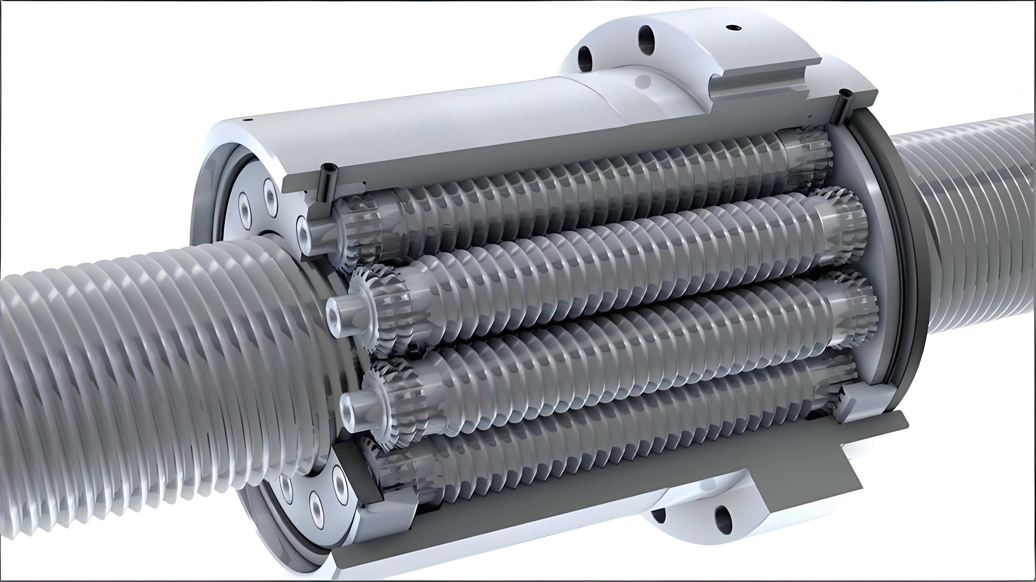
The planetary roller screw assembly (PRSA) represents a pivotal high-precision electromechanical actuator component, renowned for its exceptional load capacity, longevity, transmission accuracy, and compact design. Its operation hinges on the coordinated planetary motion of multiple threaded rollers situated between a central screw and an outer nut. The conversion between rotary and linear motion is achieved through the meshing of complementary spatial helical surfaces on these three primary components: the screw, the nut, and the rollers. A profound understanding of the kinematic behavior within this assembly is fundamental, as it directly governs critical performance metrics such as contact mechanics, friction characteristics, dynamic response, and ultimately, fatigue life. This article establishes a rigorous kinematic model based on parametric representations of the helical surfaces. Through this model, we derive the governing relationships between structural parameters, simulate spatial motion trajectories, and, most significantly, elucidate the distinct cyclic stress patterns experienced by each component. This analysis provides a theoretical foundation for life prediction and reliability-oriented design of the planetary roller screw assembly.
The kinematic integrity and force transmission of a planetary roller screw assembly depend entirely on the precise geometry of the interacting threads. Each component’s thread can be mathematically described as a spatial helical surface generated by sweeping a two-dimensional profile along a helix. To analyze the system, we define component-specific Cartesian coordinate systems. Let the z-axis coincide with the component’s axis of rotation. A point \(Q\) on any helical surface can be located by its radial distance \(r\) from the axis and its angular position \(\alpha\). Its axial coordinate \(z\) combines a function of the profile \(\phi(r)\) and the helical lead.
The general parametric equation for a helical surface in its local coordinate system \(O-xyz\) is given by:
$$\boldsymbol{\psi}(r, \alpha) = \left[ r\cos\alpha,\ r\sin\alpha,\ \zeta\phi(r) + \frac{\alpha l}{2\pi} \right]^T$$
Here, \(l\) is the lead of the thread. The Boolean variable \(\zeta\) distinguishes between the two flanks of the thread: \(\zeta = +1\) typically for one flank (e.g., the “lower” or “driving” flank) and \(\zeta = -1\) for the opposing (“upper”) flank. The partial derivatives with respect to the parameters are:
$$\boldsymbol{\psi}_r = \frac{\partial \boldsymbol{\psi}}{\partial r} = \left[ \cos\alpha,\ \sin\alpha,\ \zeta\phi'(r) \right]^T$$
$$\boldsymbol{\psi}_\alpha = \frac{\partial \boldsymbol{\psi}}{\partial \alpha} = \left[ -r\sin\alpha,\ r\cos\alpha,\ \frac{l}{2\pi} \right]^T$$
The unit normal vector pointing toward the thread interior (crucial for contact analysis) is:
$$\mathbf{n} = \zeta \frac{\boldsymbol{\psi}_r \times \boldsymbol{\psi}_\alpha}{||\boldsymbol{\psi}_r \times \boldsymbol{\psi}_\alpha||}$$
For the screw, which is a multi-start external thread with a trapezoidal profile, the profile function \(\phi_S(r_S)\) within the thread region \(d_{S2}/2 \le r_S \le d_{S1}/2\) is:
$$\phi_S(r_S) = \left( r_S – \frac{d_{S0}}{2} \right) \tan\beta_S + \frac{P_S – h_S}{2}$$
where \(d_{S0}, d_{S1}, d_{S2}\) are pitch, major, and minor diameters; \(P_S\) is the pitch; \(h_S\) is the thread thickness; \(\beta_S\) is the flank half-angle; and \(n_S\) is the number of starts (\(l_S = n_S P_S\)). The unit normal vector simplifies to:
$$\mathbf{n}_S = \zeta_S \begin{bmatrix} \dfrac{l_S \sin\alpha_S}{2\pi r_S} – \zeta_S \cos\alpha_S \tan\beta_S \\ -\dfrac{l_S \cos\alpha_S}{2\pi r_S} – \zeta_S \sin\alpha_S \tan\beta_S \\ 1 \end{bmatrix} \cdot \left[ 1 + \left(\dfrac{l_S}{2\pi r_S}\right)^2 + \tan^2\beta_S \right]^{-1/2}$$
The nut is an internal multi-start thread. Its profile function \(\phi_N(r_N)\) for \(d_{N2}/2 \le r_N \le d_{N1}/2\) is:
$$\phi_N(r_N) = \frac{P_N – h_N}{2} – \left( r_N – \frac{d_{N0}}{2} \right) \tan\beta_N$$
Its corresponding unit normal vector is:
$$\mathbf{n}_N = \zeta_N \begin{bmatrix} \dfrac{l_N \sin\alpha_N}{2\pi r_N} + \zeta_N \cos\alpha_N \tan\beta_N \\ -\dfrac{l_N \cos\alpha_N}{2\pi r_N} + \zeta_N \sin\alpha_N \tan\beta_N \\ 1 \end{bmatrix} \cdot \left[ 1 + \left(\dfrac{l_N}{2\pi r_N}\right)^2 + \tan^2\beta_N \right]^{-1/2}$$
The roller is typically a single-start external thread with a circular (arc) profile to minimize friction. The radius of the circular arc is \(R_e = d_{R0}/(2\sin\beta_R)\). Its profile function for \(d_{R2}/2 \le r_R \le d_{R1}/2\) is:
$$\phi_R(r_R) = R_e \cos\beta_R + \frac{P_R – h_R}{2} – \sqrt{R_e^2 – r_R^2}$$
The unit normal vector for the roller’s helical surface is:
$$\mathbf{n}_R = \zeta_R \begin{bmatrix} \dfrac{l_R \sin\alpha_R}{2\pi r_R} – \dfrac{\zeta_R \cos\alpha_R \cdot r_R}{\sqrt{R_e^2 – r_R^2}} \\ -\dfrac{l_R \cos\alpha_R}{2\pi r_R} – \dfrac{\zeta_R \sin\alpha_R \cdot r_R}{\sqrt{R_e^2 – r_R^2}} \\ 1 \end{bmatrix} \cdot \left[ 1 + \left(\dfrac{l_R}{2\pi r_R}\right)^2 + \dfrac{r_R^2}{R_e^2 – r_R^2} \right]^{-1/2}$$
To analyze the system kinematics, we establish a fixed global frame \(O-xyz\) that coincides with the nut’s coordinate system \(O_N-x_Ny_Nz_N\), as the nut typically translates without rotation. The screw coordinate system \(O_S-x_Sy_Sz_S\) initially aligns with the global frame and then rotates about the z-axis with an angular velocity \(\omega_S\). Each roller has a body-fixed frame \(O_R-x_Ry_Rz_R\) and undergoes a complex motion: planetary revolution about the screw axis with angular velocity \(\omega_H\) and radius \(r_H = (d_{S0}+d_{R0})/2\), and rotation about its own axis with angular velocity \(\omega_R\). Its center also translates axially along with the nut.
The absolute velocity of any point on a component is derived by differentiating its position vector in the global frame. For a point on the screw with local coordinates \((r_S, \alpha_S)\), after a rotation \(\theta_S = \omega_S t\), its velocity in the global frame is pure tangential:
$$\mathbf{v}^o_S = \left[ -r_S \omega_S \sin(\alpha_S + \theta_S),\ r_S \omega_S \cos(\alpha_S + \theta_S),\ 0 \right]^T$$
For a point on the nut \((r_N, \alpha_N)\), the velocity is purely axial, equal to the nut’s translation speed:
$$\mathbf{v}^o_N = \left[ 0,\ 0,\ -\frac{\omega_S l_S}{2\pi} \right]^T$$
The motion of a point on a roller \((r_R, \alpha_R)\) is more complex, being the sum of its relative rotation velocity within the roller-fixed frame, the translational velocity of the roller’s center, and the revolution velocity of that center. Its absolute velocity \(\mathbf{v}^o_R\) is given by:
$$
\begin{aligned}
\mathbf{v}^o_R = & \begin{bmatrix} r_R \omega_R \sin(\alpha_R – \theta_R) \\ -r_R \omega_R \cos(\alpha_R – \theta_R) \\ 0 \end{bmatrix} + \begin{bmatrix} -r_{RH} \omega_H \sin(\theta_H + \alpha_{RH}) \\ r_{RH} \omega_H \cos(\theta_H + \alpha_{RH}) \\ 0 \end{bmatrix} \\ &+ \begin{bmatrix} 0 \\ 0 \\ -\frac{\omega_S l_S}{2\pi} \end{bmatrix}
\end{aligned}
$$
where \(r_{RH}\) and \(\alpha_{RH}\) define the position of the coincident point on the revolution radius relative to the global origin, found via geometric relations in the triangle formed by the global origin, the roller center, and the point on the roller.
The core of the kinematic analysis for the planetary roller screw assembly lies in determining the contact points between the screw-roller and nut-roller interfaces and enforcing the conditions for proper meshing. According to the theory of gearing and the condition of continuous tangency, at a point of contact between two surfaces, the position vectors coincide, and the unit normals are collinear (opposite in direction).
For the screw-roller contact pair, let the contact point parameters be \((r_{Sc}, \alpha_{Sc})\) for the screw and \((r_{RSc}, -\alpha_{RSc})\) for the roller (the negative sign accounts for the opposite thread orientation relative to the screw). The following conditions must be satisfied simultaneously:
1. Position Coincidence (in the transverse plane):
$$ r_{Sc} \sin\alpha_{Sc} = r_{RSc} \sin\alpha_{RSc} $$
$$ r_{Sc} \cos\alpha_{Sc} + r_{RSc} \cos\alpha_{RSc} = \frac{d_{S0} + d_{R0}}{2} $$
2. Normal Vector Collinearity: \(\mathbf{n}_{Sc} = -\mathbf{n}_{RSc}\).
This yields two scalar equations derived from the cross-product condition, involving the leads \(l_S, l_R\), profile parameters \(\beta_S, R_e\), and the Boolean variables \(\zeta_{Sc}, \zeta_{RSc}\) (where \(\zeta_{RSc} = -\zeta_{Sc}\)).
Similarly, for the nut-roller contact pair with parameters \((r_{Nc}, \alpha_{Nc})\) for the nut and \((r_{RNc}, \alpha_{RNc})\) for the roller, the conditions are:
1. Position Coincidence:
$$ r_{Nc} \sin\alpha_{Nc} = r_{RNc} \sin\alpha_{RNc} $$
$$ r_{Nc} \cos\alpha_{Nc} – r_{RNc} \cos\alpha_{RNc} = \frac{d_{N0} – d_{R0}}{2} $$
2. Normal Vector Collinearity: \(\mathbf{n}_{Nc} = -\mathbf{n}_{RNc}\), with \(\zeta_{Nc} = \zeta_{RSc}\) and \(\zeta_{RNc} = -\zeta_{RSc}\).
Solving these four sets of equations numerically for a given planetary roller screw assembly geometry yields the precise contact point parameters. A key result from this analysis is that the screw-roller contact point generally has a non-zero contact angle (\(|\alpha_{Sc}| > 0\)), meaning the contact occurs off the line connecting their centers. In contrast, the nut-roller contact point lies precisely on the line connecting their centers (\(\alpha_{Nc} = 0, \alpha_{RNc} = 0\)), making it the instantaneous center of velocity (no relative velocity in the transverse plane) for that contact pair. The screw-roller contact point, however, exhibits a non-zero relative sliding velocity.
The kinematic constraints at the contact points, specifically the requirement that the normal components of velocity at the contacting surfaces are equal (to maintain contact), lead to the fundamental speed and geometric relationships governing the planetary roller screw assembly. Analyzing the screw-roller contact yields:
$$\frac{\omega_R}{\omega_H} = \frac{l_S}{l_R}$$
Analyzing the nut-roller contact yields:
$$\frac{\omega_R}{\omega_H} = \frac{l_N}{l_R}$$
Furthermore, from the condition at the instantaneous center (nut-roller contact), the transverse velocity balance gives:
$$\frac{\omega_R}{\omega_H} = \frac{d_{N0}}{d_{R0}}$$
Combining these and relating the screw’s rotational speed to the planetary revolution speed via the geometry of rolling leads to the complete set of design relations for a standard planetary roller screw assembly:
$$
\begin{aligned}
& k_{\omega} = \frac{d_{N0}}{d_{R0}} = \frac{l_S}{l_R} = \frac{l_N}{l_R} = \frac{\omega_R}{\omega_H} \\
& \omega_H = \frac{\omega_S (k_{\omega} – 2)}{2(k_{\omega} – 1)} \\
& \omega_R = \frac{\omega_S k_{\omega} (k_{\omega} – 2)}{2(k_{\omega} – 1)} \\
& d_{S0} = (k_{\omega} – 2) d_{R0}
\end{aligned}
$$
These equations are critical. They show that the ratio of nut-to-roller pitch diameter \(k_{\omega}\) is the key design parameter, dictating the speed ratios and the screw diameter. For proper assembly and function, \(k_{\omega}\) must be an integer, representing the number of roller thread starts (or equivalently, the number of nut thread starts). This integer defines the number of complete roller rotations per one revolution of the roller around the screw.
The motion trajectories of points on the components, especially the rollers, are complex spatial curves. While a point on the screw’s contact trace moves on a simple circle, and a point on the nut’s contact trace moves on a straight line parallel to the axis, a point on the roller’s contact trace with the nut follows a complex, spatially closed curve. During one complete revolution of the roller around the screw (period \(T_H = 2\pi/\omega_H\)), the roller completes exactly \(k_{\omega}\) rotations about its own axis (period \(T_R = 2\pi/\omega_R\)). The axial displacements per revolution are fixed by geometry:
$$ \Delta z_R = \frac{2\pi (k_{\omega} – 1) l_S}{k_{\omega} (k_{\omega} – 2)}, \quad \Delta z_H = k_{\omega} \Delta z_R $$
The roller’s spatial trajectory over one orbital period \(T_H\) consists of \(k_{\omega}\) lobes, each corresponding to one roller rotation but with slightly different shapes. The trajectory repeats perfectly every orbital period.
This precise kinematic behavior directly dictates the load and stress cycles experienced by the threads, which is paramount for fatigue life analysis of the planetary roller screw assembly. Consider a specific, fixed material point on the thread of a given component. The frequency at which this point comes into contact and bears load depends on its motion relative to the other components.
- Roller Stress Cycle: A specific point on a roller’s thread will contact either the screw or the nut periodically. The time interval between successive contacts at the same point is \(T_{Rc} = 2\pi / [\omega_H (k_{\omega}+1)]\). Under constant operational load, this point therefore experiences a steady pulsating (or alternating) cyclic contact stress with a fixed period \(T_{Rc}\). The number of stress cycles on the roller per screw revolution is \(n_{Rc} = (k_{\omega}-2)(k_{\omega}+1)/[2(k_{\omega}-1)]\).
- Nut Stress Cycle: A specific point on the nut’s internal thread is loaded each time a roller passes over it. With \(z\) rollers equally spaced, the time between successive contacts is \(T_{Nc} = 2\pi/(z \omega_H)\). Consequently, the nut thread point also endures a steady pulsating cyclic contact stress, but with a period dependent on the number of rollers. The stress cycles per screw revolution are \(n_{Nc} = z(k_{\omega}-2)/[2(k_{\omega}-1)]\).
- Screw Stress Cycle: The stress history on a specific point on the screw’s thread is more complex. This point is loaded sequentially by different rollers. The time between contacts from successive rollers is \(T_{Sc} = 2\pi/[z(\omega_S – \omega_H)]\). However, since the nut (and thus the loaded zone of engagement) translates axially along the screw, a given screw thread point will experience loading only when the nut’s travel brings a roller into engagement with it. Therefore, the load on a fixed screw point is not periodic with a simple constant period but is a periodic variable-amplitude cyclic stress. The pattern repeats over the nut’s reciprocation cycle along the screw’s effective stroke length \(l_{PRSA}\). The number of engagements per passage of the nut can be calculated based on the number of roller threads and the axial travel per roller revolution.
The distinct stress cycle behaviors for each component in a planetary roller screw assembly are summarized in the table below:
| Component | Cycle Type | Governed By | Cycles per Screw Rev. (Example) |
|---|---|---|---|
| Roller | Steady Pulsating | \(T_{Rc} = \dfrac{2\pi}{\omega_H (k_{\omega}+1)}\) | \(n_{Rc} = \dfrac{(k_{\omega}-2)(k_{\omega}+1)}{2(k_{\omega}-1)}\) |
| Nut | Steady Pulsating | \(T_{Nc} = \dfrac{2\pi}{z \omega_H}\) | \(n_{Nc} = \dfrac{z(k_{\omega}-2)}{2(k_{\omega}-1)}\) |
| Screw | Periodic Variable-Amplitude | Nut reciprocation period \(T_{PRSA}\) & engagement logic | Varies with axial position |
These stress cycle characteristics enable the prediction of the working life \(L_h\) (in hours) for the planetary roller screw assembly. The total number of stress cycles for each component over its service life is:
$$ N_{Rc} = \frac{1800 \omega_S n_{Rc} L_h}{\pi}, \quad N_{Nc} = \frac{1800 \omega_S n_{Nc} L_h}{\pi} $$
For the screw, the life calculation must account for the variable-amplitude cycle count over the nut’s reciprocation period \(T_{PRSA} = 2 l_{PRSA} / (\omega_S l_S)\). The fatigue life for each component, based on its material’s S-N curve (e.g., \(\sigma^m_{max} N = \sigma^m_0 N_0\)), can be estimated. The system’s overall life is then limited by the first component to fail:
$$ L_{life} = \min \left( \frac{N_{R}^{fatigue}}{1800 \omega_S n_{Rc}/\pi},\ \frac{N_{N}^{fatigue}}{1800 \omega_S n_{Nc}/\pi},\ \frac{T_{PRSA} N_{S}^{fatigue}}{3600 n_{Sc}} \right) $$
where \(N_{R}^{fatigue}, N_{N}^{fatigue}, N_{S}^{fatigue}\) are the allowable fatigue cycles for the roller, nut, and screw materials at their respective operating contact stresses, and \(n_{Sc}\) is the number of screw stress cycles per nut passage.
In conclusion, the kinematic analysis of a planetary roller screw assembly, rooted in the parametric description of its helical surfaces, reveals intricate motion and force transmission mechanisms. The derived relationships between pitches, diameters, and angular velocities are fundamental for design. More importantly, the kinematic model uncovers the inherent differences in stress cycle patterns: the roller and nut threads experience steady cyclic stresses, while the screw thread undergoes a complex variable-amplitude cycle due to the translating nut. This understanding is not merely academic; it provides the essential framework for accurate contact fatigue analysis, load distribution studies, dynamic modeling, and ultimately, for the reliable design and life prediction of high-performance planetary roller screw assemblies. Future work integrating these kinematic insights with nonlinear contact mechanics and system dynamics will further enhance the predictive capabilities for this critical actuator component.