
The design of spiral bevel gears is a complex engineering task characterized by numerous interdependent parameters and stringent performance constraints. Achieving an optimal design that balances weight, cost, strength, and manufacturability is challenging using conventional iterative or handbook-based methods. This article details a structured approach to formulating and solving the spiral bevel gear optimization problem, focusing on the development of a robust mathematical model and the application of a suitable discrete optimization algorithm. The primary goal is to enhance design efficiency and quality by systematically navigating the vast design space to identify the best possible configuration for a given set of requirements.
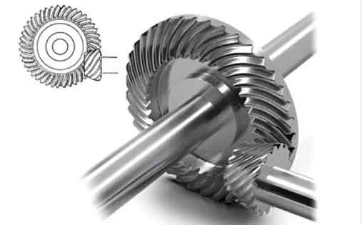
In mechanical power transmission systems, especially in reducers, spiral bevel gears are critical components for transmitting power between non-parallel, intersecting shafts. Their curved teeth allow for smoother engagement, higher load capacity, and reduced noise compared to straight bevel gears. However, this complexity translates into a multidimensional design problem. An engineer must simultaneously select discrete parameters like tooth numbers and continuous parameters like module and face width, all while ensuring the design satisfies geometric, kinematic, strength, and manufacturing limitations. Failure to properly account for any of these constraints can lead to premature failure, excessive noise, or an impractical design.
1. Selection of Optimization Algorithm for Discrete Problems
The design variables for spiral bevel gears often include inherently discrete quantities, such as the number of teeth (which must be integers) and the module (which typically follows a standard series). This characteristic places the problem within the domain of discrete or mixed-integer nonlinear programming. Common optimization algorithms include gradient-based methods, penalty function methods, and random search techniques like genetic algorithms. However, for problems where the feasible region—the set of all variable combinations satisfying all constraints—is a very small subset of the total combinatorial space, a method known as feasible enumeration proves to be exceptionally efficient.
The brute-force approach, or complete enumeration, involves listing every possible combination of design variables, calculating the objective function (e.g., gear volume) for each, and selecting the best. While guaranteed to find the global optimum, this method becomes computationally intractable for even moderately sized problems due to the explosive growth of combinations. For instance, choosing from 20 possible tooth numbers for each of two gears already yields 400 combinations before considering other variables.
Feasible enumeration intelligently prunes this search tree. Its core logic operates in two stages for each potential variable combination:
- Constraint Feasibility Check: Before any performance calculation, the combination is checked against all defined constraints (e.g., minimum tooth number, geometric compatibility). If it violates any single constraint, it is immediately discarded.
- Promising Solution Check: If the combination passes all constraints, a quick, conservative estimate is made to determine if its objective function value could potentially be better than the best value found so far. If the estimate indicates it cannot possibly improve upon the current best solution, it is also discarded.
Only those combinations that are both feasible and potentially optimal proceed to the computationally expensive steps of precise geometry generation, stress analysis, and objective function evaluation. In the design of spiral bevel gear reducers, the ratio of feasible combinations to total combinations is often extremely low. This makes feasible enumeration a powerful tool, transforming an otherwise impossible exhaustive search into a manageable process that still guarantees a globally optimal solution within the defined discrete space.
| Algorithm | Principle | Pros for Gear Design | Cons for Gear Design |
|---|---|---|---|
| Complete Enumeration | Evaluates all possible variable combinations. | Guaranteed global optimum; simple concept. | Computationally prohibitive for realistic problems. |
| Feasible Enumeration | Evaluates only feasible & promising combinations. | Finds global optimum; highly efficient for sparse feasible spaces. | Efficiency depends heavily on constraint “tightness”. |
| Gradient-Based Methods | Uses derivatives to find local improvements. | Fast convergence near an optimum. | Requires continuous variables; finds local optima; sensitive to initial guess. |
| Genetic Algorithms | Mimics natural selection using a population of designs. | Handles discrete/continuous variables; good for global search. | Computationally expensive; no guarantee of true optimum; many tuning parameters. |
2. Formulation of the Mathematical Model
The cornerstone of a successful optimization is a precise and complete mathematical model. For spiral bevel gears, this model comprises three fundamental elements: the design variables, the objective function, and the constraint functions.
2.1 Design Variables
The design variables are the independent parameters the optimization algorithm is free to adjust. Their selection is crucial and is based on a comprehensive analysis of the spiral bevel gear design process, which is governed by standards for calculating load capacity (e.g., contact and bending strength per ISO 10300 or similar). The parameters can be categorized as follows:
- Operational Conditions: Load power, input speed, service factor (KA), desired lifetime, lubricant viscosity.
- Gear Tooth System (Basic Settings): Normal pressure angle ($\alpha_n$), spiral angle ($\beta_m$), addendum coefficient ($h_a^*$), dedendum coefficient ($c^*$), cutter radius ($r_0$).
- Manufacturing & Assembly: Manufacturing quality grade, alignment errors, surface finish.
- Material & Heat Treatment: Material grade, hardness, bending and contact fatigue limits ($\sigma_{Flim}$, $\sigma_{Hlim}$).
- Key Geometrical Parameters (Primary Variables): Among these, a subset is typically chosen as active optimization variables due to their significant impact on size and performance. Common choices include:
- Number of teeth on pinion and gear ($z_1$, $z_2$) – Discrete
- Normal module at the midpoint ($m_n$) – Discrete (from standard series)
- Face width ($b$) – Continuous or discrete
- Spiral angle at the midpoint ($\beta_m$) – Continuous
- Profile shift coefficients ($x_1$, $x_2$) – Continuous
2.2 Objective Function
The objective function, $F(X)$, quantifies the goal of the optimization. For spiral bevel gear reducers, two primary objectives are prevalent:
- Minimum Volume/Weight: This is the most common goal for designing a new, dedicated reducer. Given a required power and speed, the aim is to find the lightest/smallest gears that can safely transmit the load. A suitable proxy is minimizing the sum of the volumes of the gear blanks, which is largely driven by the pitch cone dimensions. An approximate objective function can be:
$$ F_1(X) = k \cdot (d_{m1}^2 \cdot b + d_{m2}^2 \cdot b) $$
where $d_{m1}$ and $d_{m2}$ are the mean pitch diameters of the pinion and gear, $b$ is the face width, and $k$ is a constant relating to geometry. Minimizing $F_1(X)$ directly reduces material cost and inertia. - Maximum Load Capacity: This objective is used when improving an existing product or series. Given a fixed center distance or gear size, the goal is to maximize the transmissible torque or power. The objective function could be the inverse of the calculated safety factors:
$$ F_2(X) = -\min(S_H, S_F) $$
where $S_H$ and $S_F$ are the contact and bending safety factors, respectively. Maximizing the minimum safety factor ensures balanced and maximum utilization of the gearset’s potential.
2.3 Constraint Functions
Constraints define the boundary between feasible and infeasible designs. A meticulous and complete set of constraints is essential; missing one can yield an optimal design that is impractical or unsafe. The constraints for spiral bevel gears are multifaceted:
1. Discrete Value Constraints: These enforce standard or practical selections.
$$ z_1, z_2 \in \mathbb{Z}^+ \quad \text{(Positive Integers)} $$
$$ m_n \in \{ \text{Standard Module Series} \} $$
2. Geometric and Kinematic Constraints:
- Undercutting Avoidance: The pinion must have a sufficient number of teeth to avoid undercutting during generation.
$$ z_1 \geq z_{1,\min} $$ - Machine Tool Limits (e.g., Cradle Setting $R_M$): The generated gear geometry must be within the physical limits of the manufacturing machine.
$$ R_{M,\min} \leq R_M(X) \leq R_{M,\max} $$ - Spiral Angle Range: Typically constrained for smooth operation and manufacturing.
$$ \beta_{\min} \leq \beta_m \leq \beta_{\max} $$
3. Strength Constraints: These are the core performance constraints, ensuring safe operation.
- Contact (Pitting) Stress Constraint: The calculated contact stress must be less than the permissible stress.
$$ g_1(X) = \sigma_H – \sigma_{HP} \leq 0 \quad \text{or} \quad g_1′(X) = S_{H,\min} – S_H \leq 0 $$
where $\sigma_H$ is the calculated contact stress, $\sigma_{HP}$ is the allowable contact stress, and $S_H$ is the contact safety factor. - Bending (Root) Stress Constraint: The calculated root bending stress must be less than the permissible stress.
$$ g_2(X) = \sigma_F – \sigma_{FP} \leq 0 \quad \text{or} \quad g_2′(X) = S_{F,\min} – S_F \leq 0 $$
for both the pinion and the gear.
4. Transmission Ratio Constraint: The actual ratio must closely match the required ratio ($i_{req}$).
$$ g_3(X) = \left| \frac{z_2 / z_1 – i_{req}}{i_{req}} \right| – \delta_{i,\max} \leq 0 $$
where $\delta_{i,\max}$ is the maximum allowable relative deviation (e.g., 0.03 for 3%).
5. Tooth Pairing Constraints: To ensure even wear and avoid excitation of specific harmonics, the tooth numbers should preferably be coprime and not divisible by the number of cutter blade groups.
The complete optimization problem for minimum volume design can thus be stated as:
$$ \begin{aligned}
&\text{minimize} \quad F_1(X) = k \cdot (d_{m1}^2 \cdot b + d_{m2}^2 \cdot b) \\
&\text{subject to:} \\
&\quad g_j(X) \leq 0, \quad j = 1, 2, …, m \quad \text{(All inequality constraints above)} \\
&\quad x_i^{(L)} \leq x_i \leq x_i^{(U)}, \quad i = 1, 2, …, n \quad \text{(Side bounds)} \\
&\quad x_i \in \mathbb{Z} \text{ for } i \in I_d \quad \text{(Discrete variables)}
\end{aligned} $$
where $X = [z_1, z_2, m_n, b, \beta_m, …]^T$ is the vector of design variables.
3. Case Study: Minimum Volume Design for a Klingelnberg-Type Spiral Bevel Gear Set
To illustrate the practical application of the mathematical model and the feasible enumeration algorithm, consider the design of a Klingelnberg-type spiral bevel gear set for a reducer. The goal is to achieve minimum volume while transmitting a specified torque and speed.
3.1 Problem Setup and Algorithm Flow
The optimization program follows a logical sequence, as outlined in the flowchart below, which embodies the feasible enumeration strategy. The process begins by defining the search ranges for all discrete and continuous variables. It then systematically generates candidate combinations, filters them through the constraint sieve, and evaluates the objective function only for the viable, promising candidates.
Program Structure for Feasible Enumeration:
1. Define input requirements (power, speed, ratio, material).
2. Set bounds and discrete sets for $z_1$, $z_2$, $m_n$, $b$, $\beta_m$.
3. Initialize best solution: $F_{best} = \infty$.
4. FOR each combination of $(z_1, z_2, m_n)$ in their discrete sets
5. IF $z_1 < z_{1,\min}$ OR ratio error $ > \delta_{i,\max}$ THEN CONTINUE
6. IF machine setting $R_M$ is out of bounds THEN CONTINUE
7. For remaining continuous variables ($b$, $\beta_m$), check geometric bounds.
8. IF a quick volume estimate $F_{est} \geq F_{best}$ THEN CONTINUE
9. // *** Now perform full strength calculation ***
10. Calculate precise geometry, stresses $\sigma_H$, $\sigma_F$.
11. IF $\sigma_H > \sigma_{HP}$ OR $\sigma_F > \sigma_{FP}$ THEN CONTINUE
12. Calculate final objective function $F_1(X)$.
13. IF $F_1(X) < F_{best}$ THEN update $F_{best}$ and save $X_{best}$.
14. END FOR
15. Output optimal solution $X_{best}$ and performance data.
3.2 Strength Calculation and Intermediate Results
For a candidate design that passes the initial geometric filters, a full strength analysis is performed per relevant standards. A snapshot of such a calculation for a specific candidate is shown below. The algorithm checks both pitting resistance (contact stress) and bending strength at the tooth root. The design is only considered feasible if the calculated safety factors exceed the minimum allowable values (e.g., $S_H \geq 1.5$ and $S_F \geq 2.5$ for high reliability).
| Input / Calculated Parameter | Symbol | Pinion Value | Gear Value | Unit |
|---|---|---|---|---|
| Input Data | ||||
| Shaft Angle | $\Sigma$ | 90° | – | |
| Number of Teeth | $z$ | 21 | 29 | – |
| Pinion Torque | $T_1$ | 13643 | N·m | |
| Face Width | $b$ | 130 | mm | |
| Midpoint Spiral Angle | $\beta_m$ | 30° | – | |
| Contact Stress Analysis | ||||
| Nominal Contact Stress | $\sigma_{H0}$ | 410.9 | MPa | |
| Calculated Contact Stress | $\sigma_{H}$ | 757.6 | MPa | |
| Contact Fatigue Limit | $\sigma_{Hlim}$ | 1450.0 | MPa | |
| Permissible Contact Stress | $\sigma_{HP}$ | 1481.2 | 1481.2 | MPa |
| Contact Safety Factor | $S_H$ | 1.955 | – | |
| Bending Stress Analysis | ||||
| Nominal Bending Stress | $\sigma_{F0}$ | 83.34 | 88.11 | MPa |
| Calculated Bending Stress | $\sigma_{F}$ | 283.27 | 299.45 | MPa |
| Bending Fatigue Limit | $\sigma_{Flim}$ | 450.0 | MPa | |
| Permissible Bending Stress | $\sigma_{FP}$ | 836.10 | 834.41 | MPa |
| Bending Safety Factor | $S_F$ | 2.952 | 2.786 | – |
3.3 Optimization Results
After exploring the design space using the feasible enumeration algorithm, the program converges to an optimal solution. This solution represents the set of design variables that yields the minimum gear volume while satisfying every single constraint defined in the mathematical model. The output includes the final geometrical parameters and confirms that all safety factors are within the acceptable, safe range.
| Item | Parameter | Symbol | Optimal Value |
|---|---|---|---|
| 1 | Gear Type | – | Klingelnberg Spiral Bevel |
| 2 | Normal Module (Midpoint) | $m_n$ | 15.82 mm |
| 3 | Number of Teeth (Pinion) | $z_1$ | 21 |
| 4 | Number of Teeth (Gear) | $z_2$ | 29 |
| 5 | Midpoint Spiral Angle | $\beta_m$ | 30° |
| 6 | Normal Pressure Angle | $\alpha_n$ | 20° |
| 7 | Shaft Angle | $\Sigma$ | 90° |
| 8 | Transverse Module (Outer) | $m_t$ | 21.90 mm |
| 9 | Contact Safety Factor | $S_H$ | 1.96 |
| 10 | Bending Safety Factor (Pinion/Gear) | $S_F$ | 2.95 / 2.79 |
4. Conclusion
The systematic approach to spiral bevel gear optimization, centered on a rigorously defined mathematical model and powered by an efficient discrete search algorithm like feasible enumeration, offers significant advantages over traditional design methods. This methodology not only automates the search for an optimal solution but also ensures that the final design is feasible from all critical perspectives: geometric, kinematic, strength-based, and manufacturing-related. By framing the design challenge as a constrained optimization problem, engineers can move beyond satisfying mere adequacy to actively seeking the best possible configuration. This leads to tangible benefits such as reduced material usage, lower weight and inertia, improved power density, and ultimately, more reliable and cost-effective spiral bevel gear reducers. The process encapsulates deep design knowledge into a repeatable, analytical framework, enhancing both the speed and quality of the development cycle for these complex and essential mechanical components.