
As a researcher focused on gear mechanics, I have dedicated considerable effort to understanding the bending stress behavior of hyperboloidal gears. These gears, often referred to as hypoid gears, are integral to many high-performance transmission systems, such as those in automotive differentials, aerospace actuators, and industrial machinery. The unique geometry of hyperboloidal gears, characterized by offset axes and curved teeth, enables smooth power transmission and high torque capacity. However, this complexity also makes stress analysis challenging. Traditional analytical methods, rooted in beam theory or simplified formulas, frequently fall short because they cannot adequately capture the effects of manufacturing tolerances, assembly misalignments, dynamic loading, and the true three-dimensional stress state. In contrast, the Finite Element Method (FEM) offers a powerful numerical approach that can model these intricacies with high fidelity. This article presents a detailed methodology for computing the bending stress in hyperboloidal gears via FEM, emphasizing the construction of finite element models, the derivation of influence and load matrices, and the step-by-step stress calculation process. The goal is to provide a robust framework that is more accurate and reliable than conventional techniques, and which can be implemented in specialized software for practical engineering design.
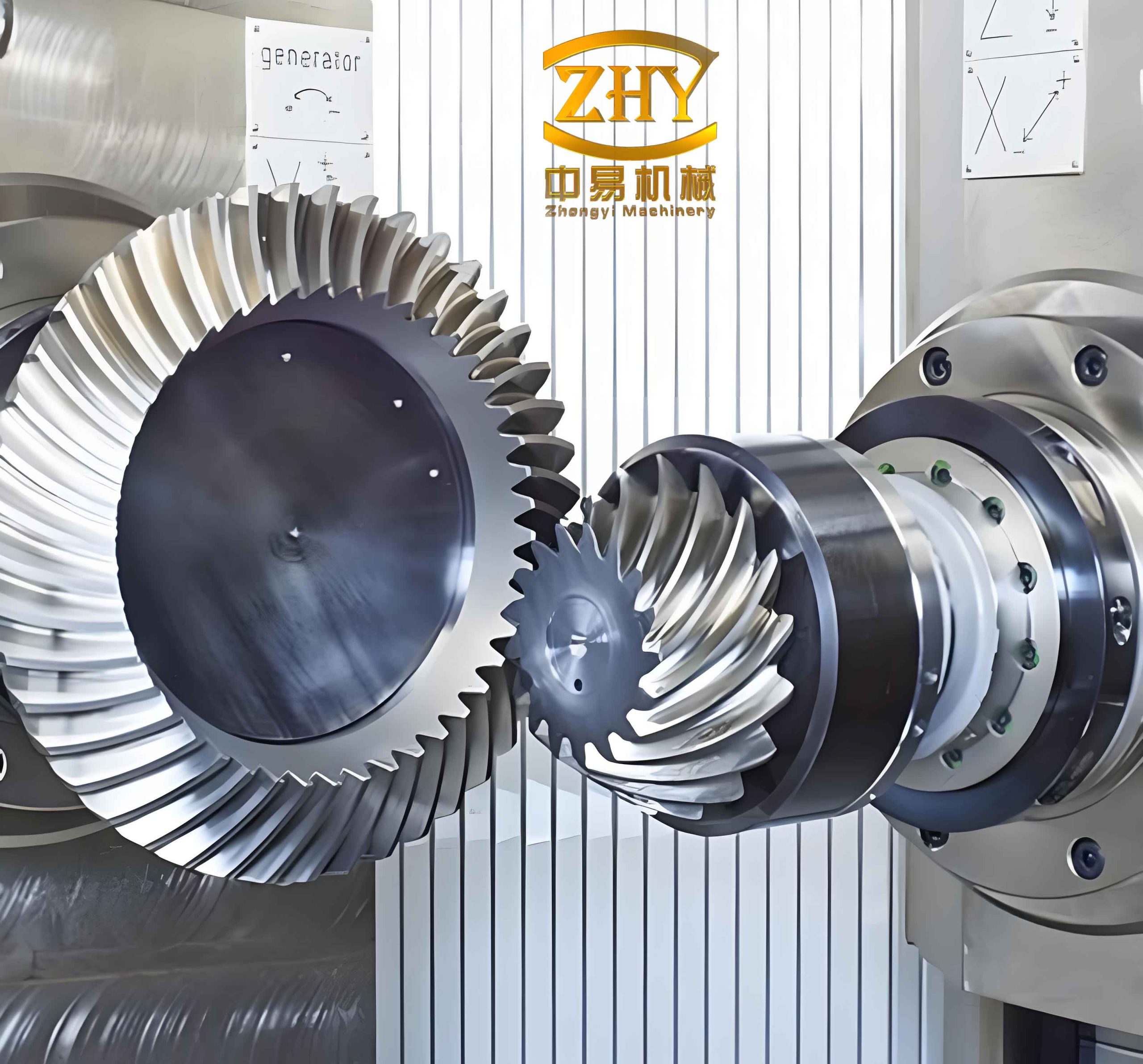
The foundation of any finite element analysis is the mesh generation. For hyperboloidal gears, creating an accurate finite element mesh requires a precise digital representation of the tooth surfaces. Given the gear pair’s geometric parameters (e.g., number of teeth, shaft angle, offset distance) and machining settings (e.g., cutter geometry, machine-tool settings), the tooth surfaces of both the pinion and the gear can be numerically simulated using mathematical models based on gear generation theory. The mesh generation procedure involves several systematic steps. First, based on computational resources and desired accuracy, the mesh density for the active tooth flanks and the critical root fillet regions is specified. Typically, a finer mesh is used in the root area where stress concentrations are expected. The mesh is initially defined on a two-dimensional projection plane related to the gear’s rotation. Imagine a coordinate system with its origin at the pitch cone apex, O, and the x-axis aligned with the gear’s rotational axis. Each prospective mesh node, i, on the tooth surface is associated with a radial distance Li from O and an angle θi measured from the x-axis. The three-dimensional coordinates (x, y, z)i of that node must satisfy the relationships tied to the gear’s conical geometry:
$$ \tan \theta_i = \frac{x_i}{\sqrt{y_i^2 + z_i^2}} $$
$$ L_i = \sqrt{x_i^2 + y_i^2 + z_i^2} $$
However, (x, y, z)i are not independent; they are functions of the intrinsic surface parameters, often denoted as u and v (or α and β), which define the tooth surface according to its equation of motion. Therefore, for each desired (Li, θi) pair from the projection plan, one must solve a system of nonlinear equations to find the corresponding surface parameters and then compute the exact spatial coordinates. This process is repeated for all nodes across the tooth surface and root fillet. Subsequently, these nodes are connected to form elements—commonly tetrahedral or hexahedral in 3D—creating the complete finite element mesh of the hyperboloidal gear tooth. The nodes on the working tooth surface are specifically flagged as potential load application points. This meticulous meshing strategy ensures that the complex curvature of hyperboloidal gears is faithfully discretized for accurate stress analysis.
A central concept in the efficient computation of bending stress for hyperboloidal gears under various load cases is the influence matrix. This matrix encodes the linear relationship between unit loads applied at any point on the tooth surface and the resulting stresses at all points in the tooth root region. Let us assume that after meshing, the total number of nodes on the combined root fillet surfaces (both driving and coast sides) is m. Consider applying a unit normal force (e.g., 1 N) at a single node i located on the working tooth surface. Solving the linear elastic finite element problem for this load case yields a stress tensor (with six components) at every node in the model. If we extract only the relevant stress component for bending (often the maximum principal stress or an equivalent stress) at each of the m root nodes, we obtain an m-dimensional vector, denoted as {S₀}ᵢ. Now, if there are k such load application nodes on the tooth surface, by applying a unit load successively at each of these k nodes, we generate k such vectors. These vectors can be assembled column-wise to form a matrix [S₀] of dimensions k × m. Each element S₀ᵢⱼ of this matrix represents the bending stress value at root node j when a unit normal load is applied at tooth surface node i. This matrix [S₀] is the full influence matrix for the tooth surface mesh nodes.
In practice, loads are not applied at arbitrary mesh nodes but are distributed over contact ellipses that move along the tooth surface during meshing. Tooth Contact Analysis (TCA) provides the path of contact and, at each discrete contact position, the orientation and dimensions of the instantaneous contact ellipse. To interface with TCA, we define a more targeted influence matrix. For a given contact position, discrete points are placed along the major axis of the contact ellipse. Suppose over all contact positions we have a total of n such discrete contact points. We can define a new influence matrix [S] of size n × m, where each element Sᵢ’ⱼ represents the bending stress at root node j when a unit normal load is applied at the i’-th discrete contact point along an ellipse major axis. The values in [S] are typically obtained by interpolating from the more comprehensive [S₀] matrix, as the discrete contact points may not coincide exactly with the original surface mesh nodes. This interpolation is a two-dimensional process considering the positions of the contact points relative to the surrounding mesh nodes on the tooth surface. The influence matrix [S] effectively serves as a pre-computed database of stress influence coefficients, dramatically speeding up stress calculations for varying load distributions.
The loading on hyperboloidal gear teeth is determined through Loaded Tooth Contact Analysis (LTCA). LTCA simulates the deformation of the gear teeth under load to compute the actual distribution of contact pressure across the contact ellipse at each meshing position. The contact pressure distribution is often elliptical (Hertzian) but can be modified by tooth modifications and system deformations. From LTCA, for a specific meshing position (say position j), we obtain a set of concentrated forces or a pressure distribution along the contact ellipse’s major axis. Discretizing this distribution yields a force vector {L}ⱼ for that position. If there are l distinct contact positions considered over the mesh cycle, and the j-th position has nⱼ discrete load points, the total number of load points is n = Σ nⱼ (for j=1 to l). All these force values can be concatenated into a single load row vector [L] of length n: [L] = [L₁, L₂, …, Lₙ]. This is the load matrix for one tooth pair under a given torque.
According to the principle of superposition, which holds for linear elastic material behavior, the total bending stress state at the root nodes is the sum of the stresses caused by each individual load. Therefore, the row vector of bending stresses at the m root nodes, denoted by [σ], is computed by a simple matrix multiplication:
$$ [\sigma]_{1 \times m} = [L]_{1 \times n} \cdot [S]_{n \times m} $$
In this equation, each element σⱼ of the resulting stress vector represents the total bending stress at root node j. The entire vector [σ] gives the stress field over the root region for that specific meshing instant. By performing this calculation for each contact position (each with its own [L] vector), we obtain a time history or load history of stress for every root node throughout the meshing cycle. This is crucial for fatigue life prediction. For each node, we have a time-varying stress signal from which we can extract amplitude and mean stress.
When multiple pairs of hyperboloidal gear teeth are in contact simultaneously—common in high-contact-ratio designs—the superposition principle extends naturally. Suppose M tooth pairs share the load at a given instant. For each pair p (p=1 to M), we have its own load vector [L]ₚ and its own influence matrix [S]ₚ (which might be identical if the teeth are symmetric, but for hyperboloidal gears, the pinion and gear teeth are different, and each tooth in a pair has its own root geometry). The total load matrix becomes a block-diagonal matrix, and the total stress at the roots of any particular tooth is influenced by loads on all contacting teeth. However, due to the localized nature of stress, the dominant contribution usually comes from the load on the tooth itself. The combined stress calculation can be expressed as:
$$ [\sigma]_{\text{total}} = \sum_{p=1}^{M} [L]_p [S]_p $$
Where the indexing is carefully managed to add stresses at corresponding root nodes of the tooth of interest.
The step-by-step algorithm for computing the bending stress in hyperboloidal gears using this influence matrix method is as follows:
- Geometry and Mesh Generation: Input the gear design parameters. Generate the precise tooth surface coordinates numerically. Create a finite element mesh for a representative tooth (or segment) of both the pinion and gear, ensuring adequate refinement at the root fillet.
- Unit Load Solutions and Influence Matrix [S₀] Calculation: For each node on the working tooth surface (or a selected subset), apply a unit normal force. Perform a linear static finite element analysis for each case. Extract the bending stress (e.g., von Mises stress or maximum principal stress) at all root fillet nodes. Compile these results into the full influence matrix [S₀].
- Tooth Contact Analysis (TCA): Perform unloaded TCA to determine the contact path, the instantaneous contact ellipse orientation, dimensions, and location for discrete roll angle positions.
- Loaded Tooth Contact Analysis (LTCA): For each TCA position, apply the intended operating torque. Solve the contact problem considering tooth flexibility (often using the flexibility matrix derived from the FEM model) to obtain the contact pressure distribution. Discretize this pressure into a set of concentrated forces at points along the contact ellipse major axis, forming the load vector [L] for each position.
- Interpolation to Form [S]: For the discrete contact points defined in LTCA, interpolate stress influence coefficients from the nearby nodes in the [S₀] matrix to construct the contact-level influence matrix [S].
- Stress Superposition: For each meshing position, compute the root stress vector using [σ] = [L][S]. Repeat for all positions to build the stress history for each root node.
- Stress Synthesis and Fatigue Assessment: At each root node, process the stress history to find the maximum stress, the stress range, and the mean stress. Use an appropriate fatigue criterion (e.g., modified Goodman, Gerber) to assess the safety factor against bending fatigue failure.
This algorithm efficiently decouples the expensive finite element solves (done once to build [S₀]) from the numerous load cases explored during LTCA and meshing analysis. It allows for rapid parametric studies, such as investigating the effect of misalignment or load variation on the bending stress of hyperboloidal gears.
To illustrate the method, consider a concrete example of a hyperboloidal gear pair used in an automotive differential. The key blank parameters are listed in the table below. These parameters define the size, shape, and relative positioning of the gears.
| Parameter | Pinion (Driving) | Gear (Driven) |
|---|---|---|
| Number of Teeth (z) | 7 | 40 |
| Shaft Angle (Σ) | 90° | 90° |
| Offset Distance (E) | 30 mm | 30 mm |
| Pitch Cone Angle (δ) | 11° 8′ 37″ | 78° 37′ 59″ |
| Face Width (b) | 51.675 mm | 47 mm |
| Outer Pitch Diameter | 22.736 mm | 299.802 mm |
| Addendum (ha) | 3.548 mm | 1.659 mm |
| Dedendum (hf) | 11.032 mm | 13.073 mm |
| Spiral Angle at Midpoint | 50° (Left-hand) | 30° (Right-hand) |
| Material | Case-Hardened Steel (Young’s Modulus E = 210 GPa, Poisson’s ratio ν = 0.3) | |
Using these parameters, the finite element models were constructed. The pinion model consisted of approximately 150,000 tetrahedral elements, with heavy refinement in the root region. The gear tooth model was similarly detailed. The unit load analyses were performed to build the influence matrices. A torque of 200 Nm was applied to the gear (input torque at the pinion correspondingly higher due to ratio). LTCA was conducted for 10 discrete contact positions across the face width from heel to toe. The resulting maximum bending stresses at the critical root fillet of the pinion and gear were computed. The stress distribution showed a characteristic pattern, with the highest stresses occurring at the root on the concave side of the tooth, slightly towards the heel end for this design. The peak von Mises equivalent stress values were found to be:
$$ \sigma_{\text{max, pinion}} \approx 450\,\text{MPa} $$
$$ \sigma_{\text{max, gear}} \approx 380\,\text{MPa} $$
These values can be compared against the material’s endurance limit to evaluate safety. Furthermore, the stress history revealed that each root node experiences a single major stress peak per mesh cycle, as expected for low-contact-ratio gearing. The influence of the offset distance, a key feature of hyperboloidal gears, on bending stress is particularly interesting. A parametric study was conducted by varying the offset while keeping other parameters constant. The results are summarized in Table 2.
| Offset Distance E (mm) | Pinion Max Stress (MPa) | Gear Max Stress (MPa) | Remarks on Contact Pattern |
|---|---|---|---|
| 25 | 420 | 360 | Contact centered, mild stress. |
| 30 (Nominal) | 450 | 380 | Contact slightly towards toe on pinion. |
| 35 | 485 | 410 | Contact shifted further, higher sliding. |
| 40 | 520 | 440 | Risk of edge loading at toe. |
This table clearly shows that increasing the offset distance in hyperboloidal gears generally increases the maximum bending stress. This is due to changes in the relative curvature and sliding conditions at the contact, which alter the load distribution and the leverage arm for root bending. Such insights are invaluable for optimizing the design of hyperboloidal gears for specific applications.
The mathematical core of the stress calculation involves tensor operations. In the finite element analysis, for each load case, the solver computes the full stress tensor at each integration point or node. For a general 3D state of stress, the tensor is:
$$ \boldsymbol{\sigma} = \begin{bmatrix} \sigma_{xx} & \tau_{xy} & \tau_{xz} \\ \tau_{yx} & \sigma_{yy} & \tau_{yz} \\ \tau_{zx} & \tau_{zy} & \sigma_{zz} \end{bmatrix} $$
For bending fatigue assessment, a scalar equivalent stress is often required. The von Mises stress, suitable for ductile materials like gear steels, is calculated as:
$$ \sigma_{\text{vM}} = \sqrt{ \frac{1}{2} \left[ (\sigma_{xx}-\sigma_{yy})^2 + (\sigma_{yy}-\sigma_{zz})^2 + (\sigma_{zz}-\sigma_{xx})^2 + 6(\tau_{xy}^2 + \tau_{yz}^2 + \tau_{zx}^2) \right] } $$
This is the value typically stored in the influence matrix and used in the subsequent superposition. For high-cycle fatigue analysis, the stress amplitude (σₐ) and mean stress (σ_m) are derived from the time history of σ_vM at each node. The modified Goodman criterion is then applied:
$$ \frac{\sigma_a}{S_e} + \frac{\sigma_m}{S_u} = \frac{1}{n} $$
where S_e is the corrected endurance limit of the gear material, S_u is the ultimate tensile strength, and n is the safety factor. Designing hyperboloidal gears requires ensuring n > 1 for all critical root locations.
One of the significant advantages of this FEM-based approach is its ability to incorporate real-world imperfections. Manufacturing errors, such as tooth profile deviations or lead crowning inaccuracies, can be introduced as modifications to the theoretical tooth surface coordinates during the mesh generation phase. Assembly errors, like misalignment of the pinion and gear axes (offset error, shaft angle error), can be directly input into the TCA and LTCA modules. The influence matrix method remains valid because the unit load solutions already reflect the tooth’s intrinsic flexibility and geometry. The load vector [L] from LTCA will automatically account for these errors by producing a different contact pressure distribution. Thus, the computed bending stress will reflect the degraded conditions, allowing engineers to assess robustness and set appropriate tolerance limits.
In terms of computational implementation, the entire process can be structured into modular software components: a geometry engine for hyperboloidal gear generation, a finite element solver (or an interface to a commercial solver like ANSYS or Abaqus), a TCA/LTCA module, and a post-processing module for stress synthesis and fatigue evaluation. Such specialized software makes this advanced analysis accessible without requiring every engineer to be an expert in finite element modeling, thus benefiting small and medium-sized enterprises that design and manufacture hyperboloidal gears.
In conclusion, the finite element method, particularly when streamlined using pre-computed influence matrices, provides a superior methodology for calculating bending stress in hyperboloidal gears. It transcends the limitations of traditional rating methods by accurately modeling complex geometry, material behavior, load sharing, and system deformations. The detailed procedure outlined here—from mesh generation and influence matrix derivation to load distribution analysis and stress superposition—offers a comprehensive and practical framework. The included example and parametric study demonstrate the method’s utility in gaining deep insights into the behavior of hyperboloidal gears under load. As the demand for efficient, compact, and high-torque transmissions grows, the accurate stress analysis of hyperboloidal gears will remain a cornerstone of reliable design. Continued advancements in computational power and algorithms will further refine this process, enabling even more sophisticated optimization of hyperboloidal gears for performance, weight, and durability.