Conjugate Rigid Wheel Design for Strain Wave Gears via Envelope Simulation

The pursuit of high-performance, compact, and precise power transmission systems has consistently driven innovation in gear design. Among the various solutions, the strain wave gear, also commonly referred to as a harmonic drive, stands out for its exceptional capabilities. Its unique operating principle, relying on the controlled elastic deformation of a flexible spline, enables remarkable advantages such as high single-stage reduction ratios, zero-backlash operation, high torque capacity, and compact coaxial configuration. These attributes make the strain wave gear indispensable in advanced applications including robotic joints, aerospace actuators, and precision optical positioning systems.

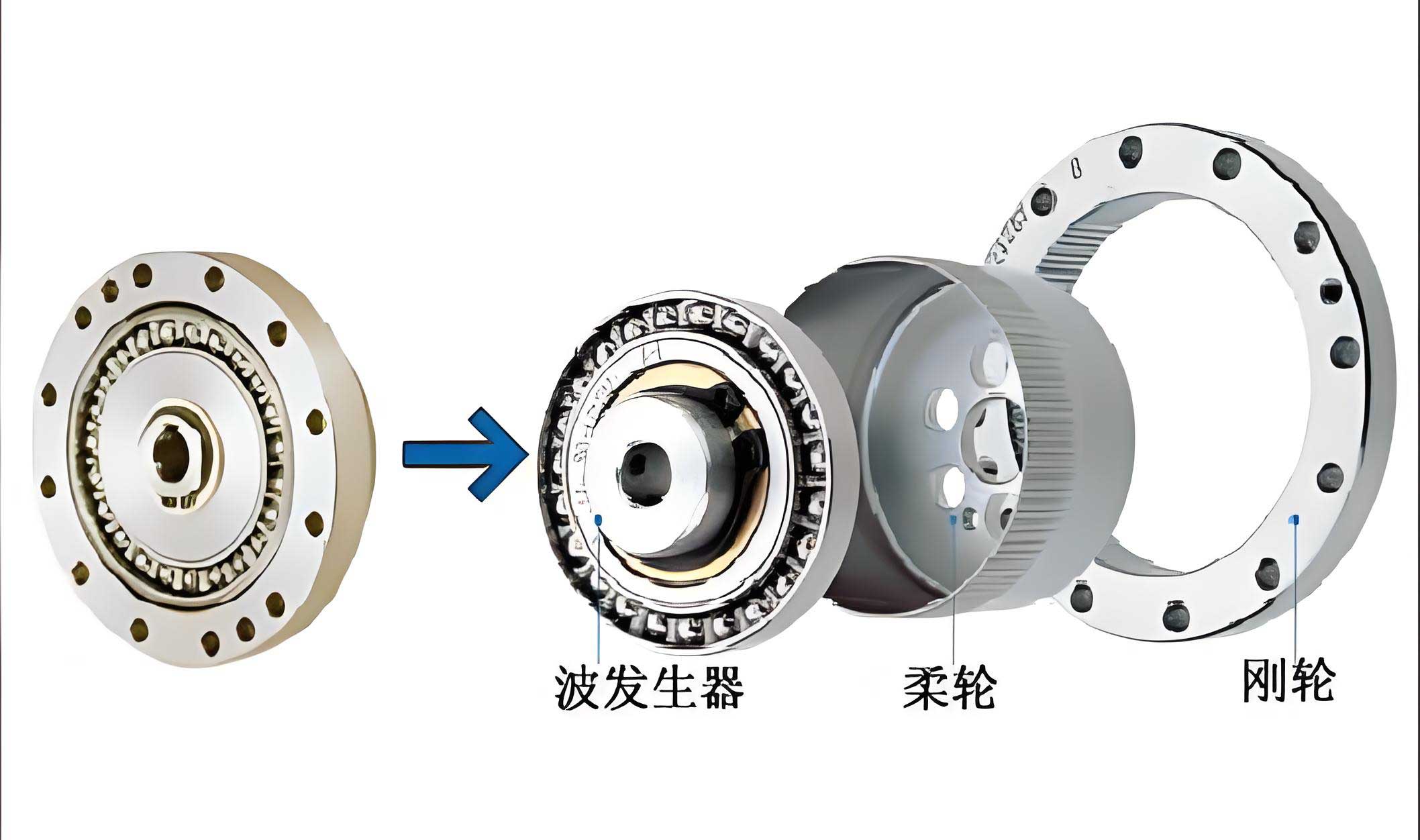
The fundamental components of a strain wave gear set are threefold: the wave generator, the flexspline (or flexible cup), and the circular spline (or rigid wheel). The wave generator, typically an elliptical ball bearing or a multi-lobed cam, is the input member. It is inserted into the flexspline, causing its initially cylindrical body to deflect into an elliptical shape. This controlled deformation forces the external teeth of the flexspline to engage with the internal teeth of the stationary circular spline at two diametrically opposite regions along the major axis of the ellipse. As the wave generator rotates, the points of engagement travel, producing a slow relative rotation between the flexspline and the circular spline. The kinematic relationship dictates that for each full revolution of the wave generator, the flexspline rotates backward by a small angle relative to the circular spline, determined by the difference in the number of teeth between the two splines.

While the principles are well-established, the design and manufacturing of high-performance strain wave gear sets remain challenging. A critical aspect is determining the precise conjugate tooth profile for the circular spline that ensures optimal meshing with a given flexspline profile under dynamic deformation. Traditional design methods often treat the flexspline and circular spline profiles somewhat independently, leading to iterative prototyping and tuning phases, which are time-consuming and costly. Furthermore, the advent of advanced finite element analysis (FEA) for stress, contact, and dynamic simulation necessitates accurate three-dimensional digital models. Existing parametric modeling tools often lack the flexibility to handle non-standard tooth profiles, such as double-arc or modified involute shapes commonly used in high-performance strain wave gears.

This article presents a comprehensive methodology for designing the conjugate tooth profile of the circular spline in a strain wave gear using a numerical envelope simulation approach. The core idea is to treat the known flexspline tooth profile as a cutting tool that moves according to the kinematic and deformation rules of the strain wave gear assembly. The envelope of all positions occupied by this “tool” defines the required conjugate profile of the circular spline. I will detail the underlying conjugate theory, implement the simulation in a computational environment, analyze the critical influence of design parameters, and demonstrate the complete workflow from simulation to 3D model generation.

Theoretical Foundation: Kinematics and Conjugate Condition

The design of conjugate profiles is rooted in the gearing theory and the specific motion of the flexspline. For a standard configuration where the circular spline is fixed, the wave generator is the input, and the flexspline is the output, the motion of the flexspline relative to the circular spline is a combination of rotation and radial deformation. To analyze this, we define two coordinate systems, as shown in the derivations from the referenced work.

The flexspline profile is designed in its own coordinate system $ (x_R, y_R) $, where the $ x_R $-axis coincides with the neutral curve of the flexspline and the $ y_R $-axis aligns with the tooth symmetry line. The circular spline coordinate system $ (x_G, y_G) $ is centered at the rotation axis of the wave generator $ O_G $, with its $ x_G $-axis aligned along the major axis of the deformed flexspline.

As the wave generator rotates, the flexspline undergoes a complex motion. Its position and orientation in the circular spline coordinate system can be described by a homogeneous transformation matrix $ \mathbf{M} $. This matrix accounts for both the rotation $ \phi $ of the flexspline’s coordinate system and the radial displacement $ \rho $ of its neutral curve points. The parameter $ \gamma $ represents the kinematic phase difference between the wave generator’s rotation and the effective rotation of the flexspline’s neutral curve, stemming from the pure rolling condition between the two splines.

The transformation from the flexspline coordinates $ (x_R, y_R) $ to the circular spline coordinates $ (x_G, y_G) $ for a given point on the flexspline tooth profile is given by:

$$
\begin{bmatrix} x_G(\theta, \varphi_1) \\ y_G(\theta, \varphi_1) \\ 1 \end{bmatrix} = \mathbf{M}(\varphi_1) \begin{bmatrix} x_R(\theta) \\ y_R(\theta) \\ 1 \end{bmatrix} = \begin{bmatrix} \cos\phi & \sin\phi & \rho \sin\gamma \\ -\sin\phi & \cos\phi & \rho \cos\gamma \\ 0 & 0 & 1 \end{bmatrix} \begin{bmatrix} x_R(\theta) \\ y_R(\theta) \\ 1 \end{bmatrix}
$$

In this equation, $ \theta $ is the parameter defining a point on the flexspline tooth profile, and $ \varphi_1 $ is the angular position of the wave generator (or equivalently, the angular parameter along the flexspline’s neutral curve from the major axis). The radial displacement $ \rho(\varphi_1) $ is defined by the shape of the wave generator. For a classical elliptical generator with semi-major axis $ a $ and semi-minor axis $ b $, the radial distance to the flexspline’s neutral curve is:

$$
\rho(\varphi_1) = \frac{ab}{\sqrt{b^2 + (a^2 – b^2) \sin^2 \varphi_1}}
$$

The angles $ \phi $ and $ \gamma $ are derived from the gearing condition and the geometry of the neutral curve. The pure rolling condition, which assumes no sliding at the pitch curve, states that the arc length traveled by a point on the flexspline’s neutral curve must equal the arc length traveled by the corresponding point on the circular spline’s pitch circle of radius $ r_G $. This leads to the integral relationship for the rotation $ \varphi_2 $ of the circular spline’s equivalent point:

$$
\int_0^{\varphi_1} \sqrt{(\rho’)^2 + \rho^2} \, d\varphi = r_G \varphi_2
$$

Consequently, the phase difference $ \gamma $ and the orientation angle $ \phi $ are:

$$
\gamma(\varphi_1) = \varphi_1 – \varphi_2 = \varphi_1 – \frac{1}{r_G} \int_0^{\varphi_1} \sqrt{(\rho’)^2 + \rho^2} \, d\varphi
$$

$$
\phi(\varphi_1) = \arctan\left(\frac{\rho'(\varphi_1)}{\rho(\varphi_1)}\right) + \gamma(\varphi_1)
$$

The family of curves generated by transforming the flexspline profile for all values of $ \varphi_1 $ is described by $ \mathbf{r}_G(\theta, \varphi_1) $. The envelope of this family, which constitutes the conjugate circular spline tooth profile, is found by solving the equation where the Jacobian of the transformation vanishes. This is the standard condition for an envelope:

$$
\frac{\partial x_G}{\partial \varphi_1} \frac{\partial y_G}{\partial \theta} – \frac{\partial y_G}{\partial \varphi_1} \frac{\partial x_G}{\partial \theta} = 0
$$

Solving this system analytically for complex tooth profiles is often intractable. Therefore, a numerical simulation-based approach, the envelope method, becomes highly advantageous.

Numerical Envelope Simulation Methodology

The numerical envelope method simulates the relative motion of the flexspline tooth as it engages with the circular spline. Conceptually, for a fine sequence of wave generator positions (i.e., discrete values of $ \varphi_1 $), the entire flexspline tooth profile is calculated and plotted in the fixed circular spline coordinate system. The outer envelope of the resulting cluster of curves represents the tooth space of the circular spline. I implemented this process using MATLAB, which provides powerful tools for matrix computation, iterative loops, and graphical visualization.

The simulation requires the following primary inputs:

Flexspline Tooth Profile Data: A set of discrete points $ (x_R(\theta_i), y_R(\theta_i)) $ defining the tooth flank, tip, and root. For this study, a double-arc profile commonly used in high-performance strain wave gears was employed.
Wave Generator Geometry: The semi-major axis $ a $ and semi-minor axis $ b $.
Gearing Parameters: The nominal module $ m $, number of teeth on the flexspline $ N_f $ and circular spline $ N_c $, and the nominal pitch radius $ r_G $ of the circular spline.

A crucial design parameter that emerges is the radial deformation coefficient $ \omega^* $. It is defined as the ratio of the maximum radial deflection of the flexspline $ \omega $ to the gear module $ m $:

$$
\omega^* = \frac{\omega}{m}
$$

Where the maximum radial deflection $ \omega = a – r $, and $ r $ is the nominal radius of the undeformed flexspline (approximately its pitch radius). This coefficient fundamentally influences the depth of engagement and the meshing mechanics. The simulation program was structured with the following logical flow, which aligns with the kinematic decomposition described earlier:

Simulation Algorithm Workflow:

Initialization: Define parameters $ a, b, m, N_f, N_c, r, r_G $. Calculate $ \omega^* $. Discretize the wave generator rotation into $ K $ steps over a 90° arc (from the major axis to the minor axis), corresponding to the engagement zone: $ \varphi_1^{(k)} = (k/K) \cdot (\pi/2), k = 0, 1, …, K $.
Kinematic Transformation Loop: For each $ \varphi_1^{(k)} $:
1. Compute the instantaneous radial displacement $ \rho^{(k)} $ using the wave generator ellipse equation.
2. Numerically evaluate the integral for $ \gamma^{(k)} $ (e.g., using the trapezoidal rule).
3. Compute the orientation angle $ \phi^{(k)} $.
4. Construct the transformation matrix $ \mathbf{M}^{(k)} $.
5. Transform every point $ (x_R(\theta_i), y_R(\theta_i)) $ on the flexspline tooth profile to the global coordinate system: $ (x_G^{(i,k)}, y_G^{(i,k)}) = \mathbf{M}^{(k)} \cdot (x_R(\theta_i), y_R(\theta_i), 1)^T $.
6. Store or plot the set of transformed points for this $ k $-th position.
Envelope Generation: After processing all $ K $ positions, a dense cluster of curves representing the “swept volume” of the flexspline tooth is generated. The envelope is visually identified as the outermost boundary of this cluster that forms a smooth, continuous tooth space profile for the circular spline.

Results: Influence of Radial Deformation Coefficient and Profile Extraction

The envelope simulation provides clear visual and quantitative insights into the meshing process. The most significant finding is the profound impact of the radial deformation coefficient $ \omega^* $ on the generated conjugate profile and the meshing characteristics. I conducted simulations for three representative values: $ \omega^* = 0.8 $ (under-deflection), $ \omega^* = 1.0 $ (standard design), and $ \omega^* = 1.2 $ (over-deflection).

Case 1: Standard Design ($ \omega^* = 1.0 $)
The envelope forms a well-defined, smooth tooth space. The cluster of curves shows a consistent pattern where multiple flexspline positions contribute to the formation of the final envelope, indicating a healthy contact zone and a progressive load sharing among teeth.

Case 2: High Radial Deformation ($ \omega^* = 1.2 $)
Increasing $ \omega^* $ increases the depth to which the flexspline tooth penetrates into the circular spline space. The envelope simulation reveals two critical effects:

The number of flexspline position curves that actively contribute to the final envelope boundary decreases. This suggests a reduction in the effective contact zone or the arc of action.
During the disengagement phase (near the minor axis), a significant gap appears between the tip of the flexspline tooth and the root of the generated circular spline profile. This large clearance increases the risk of tooth jumping or loss of contact under light load or reversal conditions, which is detrimental to positioning accuracy.

Case 3: Low Radial Deformation ($ \omega^* = 0.8 $)
Decreasing $ \omega^* $ brings the wave generator shape closer to a circle. The simulation results show:

The envelope is formed by a much larger number of flexspline position curves, implying a longer path of contact and potentially higher contact ratio, which can smooth out transmission errors.
However, the clearance between the flexspline tooth tip and the circular spline tooth root becomes very small at disengagement. This minimal clearance poses a high risk of interference or tip-to-root contact, leading to increased wear, noise, and potential binding of the mechanism.

The effects are summarized in the table below:

*Radial Deformation Coefficient ($ \omega^ $)**	Effective Contact Zone	Tip-Root Clearance at Disengagement	Primary Risk
0.8 (Low)	Widest / Longest	Very Small / Critical	Interference and Binding
1.0 (Standard)	Optimal / Well-balanced	Adequate	Minimal (Design Target)
1.2 (High)	Narrowed / Reduced	Excessively Large	Tooth Jumping and Backlash

Based on this analysis, the recommended practical range for $ \omega^* $ to avoid both interference and jumping is between 0.8 and 1.2, with the optimal value typically centered around 1.0, subject to specific application requirements regarding torque, stiffness, and accuracy.

From Simulation to 3D Model: Curve Fitting and CAD Integration

The graphical envelope is a set of discrete points. To create a manufacturable CAD model, this point cloud must be converted into a smooth, continuous curve. The procedure involves the following steps:

1. Envelope Data Point Extraction:
The simulated cluster contains points from all flexspline positions. To extract only the points constituting the envelope profile, the data is processed along the $ x_G $-axis (or angular equivalent). For a series of closely spaced $ x $-coordinates, the point with the maximum $ y $-coordinate value is identified. Collectively, these $ (x_{G_{max}}, y_{G_{max}}) $ points describe the boundary of the circular spline tooth space. This process effectively “slices” the cluster vertically and picks the topmost point at each slice.

2. Curve Fitting:
The extracted points are then fitted with a smooth curve. A simple polynomial fit can induce unwanted oscillations (Runge’s phenomenon). Therefore, a weighted smoothing spline fit is preferable. This method minimizes a function that balances the fidelity to the data (sum of squared errors) with the smoothness of the curve (integral of the squared second derivative). In MATLAB, this can be achieved using the `fit` function with a smoothing spline option or the `csaps` function for cubic smoothing splines. The resulting fitted spline provides a high-fidelity, analytical representation of the conjugate tooth profile.

3. CAD Model Generation:
The fitted spline data, representing one side of the tooth space, is exported in a standard format (e.g., IGES, STEP, or simply as a set of refined points). This data is imported into a 3D CAD system like Creo Parametric or SolidWorks. The typical workflow within CAD is:

Create a sketch on the frontal plane and import/construct the fitted curve.
Mirror the curve about the tooth centerline to form the complete tooth space profile.
Use a circular pattern to replicate the tooth space around the full 360 degrees, based on the number of circular spline teeth $ N_c $.
Extrude the profile to the desired face width of the strain wave gear circular spline, adding any necessary hub features, mounting holes, and chamfers.

This process results in a precise 3D solid model of the circular spline that is perfectly conjugate to the given flexspline profile and wave generator geometry. This model is immediately usable for subsequent digital prototyping, interference checking, and as a high-quality geometry input for finite element analysis to study mesh stresses, fatigue life, and dynamic behavior.

Discussion and Advantages of the Envelope Simulation Method

The envelope simulation method for designing strain wave gear circular splines offers distinct advantages over traditional and purely parametric approaches.

1. Fidelity to Physical Kinematics: The method directly incorporates the exact kinematic motion and deformation of the flexspline as dictated by the wave generator’s shape. It does not rely on simplified approximations of the meshing process, leading to a conjugate profile that reflects true operating conditions.

2. Flexibility and Generality: It is completely agnostic to the specific geometry of the flexspline tooth profile. Whether the profile is an involute, double-arc, triangle, or any other custom shape, the same simulation procedure applies. This makes it an invaluable tool for researching and optimizing novel tooth profiles for strain wave gears.

3. Insightful Parameter Analysis: As demonstrated, the simulation visually and quantitatively reveals the impact of key design parameters like the radial deformation coefficient $ \omega^* $. Designers can rapidly iterate through different values of $ a $, $ b $, and profile modifications to assess their effect on the contact pattern, clearance, and potential for interference or jumping before any physical part is manufactured.

4. Seamless Digital Integration: The method creates a direct digital thread from the initial design parameters to the final 3D CAD model. This streamlines the product development cycle, enabling rapid prototyping, accurate performance simulation via FEA, and facilitating direct integration with CAM software for manufacturing.

5. Educational Value: The simulation provides an excellent visual aid for understanding the complex meshing action in a strain wave gear, showing how the traveling wave of deformation engages the teeth.

Conclusion

In this article, I have presented a robust and efficient methodology for designing the conjugate circular spline tooth profile in a strain wave gear using numerical envelope simulation. The process begins with the fundamental kinematic and geometric relationships governing the gear set, which are then implemented in a computational environment like MATLAB. The core of the method simulates the flexspline tooth’s motion as it is deformed by the wave generator, and the outer envelope of this motion defines the required circular spline tooth space.

The investigation highlights the critical role of the radial deformation coefficient $ \omega^* $, demonstrating that its value must be carefully chosen within a practical range (approximately 0.8 to 1.2) to avoid the dual pitfalls of tooth interference and tooth jumping. The envelope simulation provides a clear visual means to make this assessment.

Furthermore, the workflow extends beyond simulation to practical implementation. By extracting and fitting the envelope data, a precise curve is obtained and can be directly imported into CAD software to generate a ready-to-manufacture 3D model of the circular spline. This integrated digital approach significantly enhances design efficiency, accuracy, and flexibility compared to traditional iterative methods, particularly for non-standard tooth profiles. It serves as a powerful tool for advancing the design and optimization of high-performance strain wave gear systems across various demanding engineering applications.