
1. Introduction
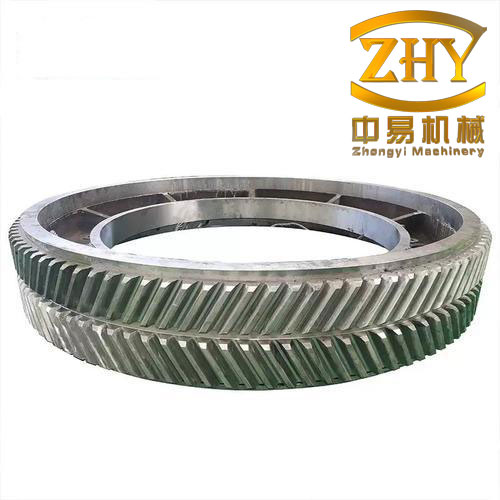
Herringbone gears are extensively employed in heavy-duty transmission systems, including marine propulsion, aerospace actuation, and high-power energy equipment, because of their high load-carrying capacity, excellent meshing stability, and the inherent cancellation of axial thrust forces. A herringbone gear can be conceptually regarded as a combination of two helical gears with opposite helix directions, separated by a central gap known as the gap width or run-out groove. During manufacturing, the two helical sides of a herringbone gear are typically machined in separate operations, which inevitably introduces manufacturing errors. Among these, the centring error is particularly characteristic of herringbone gears, defined as the offset between the two helical gear flanks along the axial direction. Additionally, due to the relatively large face width of herringbone gears, they are highly sensitive to angular misalignment errors during assembly. These errors lead to an uneven load distribution—often termed eccentric load—between the left and right helical flanks, which significantly increases contact stresses on one side and thereby diminishes the fatigue strength of the gear pair.
The prediction of contact fatigue life is crucial for the design and reliability assessment of herringbone gears. Contact fatigue failure, commonly observed as pitting or spalling, is a dominant failure mode under high-load operating conditions. The crack initiation phase typically represents the majority of the total fatigue life. The stress state beneath the tooth flank during meshing is multiaxial and generally non-proportional, as the shear stress and normal stress peaks do not occur simultaneously. Hence, employing a multiaxial fatigue criterion rooted in the critical plane concept is a more accurate approach for life estimation.
This work establishes a comprehensive computational framework for predicting the contact fatigue life of herringbone gears under the influence of centring error and two types of angular misalignment. I combined finite element contact analyses with a critical plane-based multiaxial fatigue model to capture the fatigue crack initiation life. Furthermore, I propose a semi-analytical method based on the potential energy principle to determine the eccentric load coefficients for herringbone gears with errors. The method is efficient and aligns well with numerical results, offering an effective tool for engineering design. In the remainder of this article, I discuss gear geometric modelling, finite element analysis, the fatigue life model, parametric studies on gear life, and the calculation of eccentric load coefficients with parametric sensitivity analysis.
2. Geometric Modelling and Finite Element Contact Analysis
2.1 Gear Tooth Surface Equation
Accurate geometric modelling forms the basis for reliable contact analysis. Based on the generating principle of involute gears, I derived the mathematical representation of the herringbone gear tooth flank. A rack cutter with a straight-sided profile is used to generate the involute profile, while the tooth root transition curve originates from the tip rounding of the tool. The coordinate transformation between the rack cutter coordinate system \(C_d(X_d, Y_d)\) and the gear blank coordinate system \(C_g(X_g, Y_g)\) is given by:
\[
\begin{bmatrix}
x_g \\
y_g \\
1
\end{bmatrix}
=
\begin{bmatrix}
\cos\varphi & \sin\varphi & r(\cos\varphi + \varphi\sin\varphi) \\
-\sin\varphi & \cos\varphi & r(\sin\varphi – \varphi\cos\varphi) \\
0 & 0 & 1
\end{bmatrix}
\begin{bmatrix}
x_d \\
y_d \\
1
\end{bmatrix}
\]
where \(\varphi\) is the gear rotation angle, and \(r\) is the pitch circle radius. By applying the meshing conditions and equations for the rack profile, I obtained the tooth root transition curve as:
\[
\begin{cases}
x = r(\cos\varphi + \varphi\sin\varphi) – x_c\cos\varphi – (y_c – r\varphi)\sin\varphi \\
y = r(\sin\varphi – \varphi\cos\varphi) – x_c\sin\varphi + (y_c – r\varphi)\cos\varphi
\end{cases}
\]
Using the straight rack profile, the involute curve equation is:
\[
\begin{cases}
x = r \left[ \cos\varphi + \varphi\sin\varphi – \frac{x_c + r\varphi}{r} \sin\varphi \right] \\
y = r \left[ \sin\varphi – \varphi\cos\varphi + \frac{x_c + r\varphi}{r} \cos\varphi \right]
\end{cases}
\]
The tooth flank of a helical gear is generated by sweeping the involute profile along a helix. The herringbone gear flank is obtained by the symmetric replication of the helical tooth flank across the central gap plane. The active flank surface is expressed as:
\[
\begin{cases}
X = R \cos \left( t + \frac{b \tan\beta}{r} \right) \\
Y = R \sin \left( t + \frac{b \tan\beta}{r} \right) \\
Z = \pm L_{\text{an}} + b t
\end{cases}
\]
where \(R=\sqrt{x^2+y^2}\), \(b\) is the face width of each helical side, \(L_{\text{an}}\) is the gap width, and \(\beta\) is the helix angle. Table 1 lists the basic parameters of the herringbone gear pair used throughout this study.
Table 1 Basic parameters of herringbone gear pair
| Parameter | Unit | Pinion | Gear |
|—|—|—|—|
| Number of teeth | – | 37 | 79 |
| Normal module | mm | 2.5 | 2.5 |
| Normal pressure angle | ° | 20 | 20 |
| Helix angle | ° | 15 | 15 |
| Face width per side | mm | 105 | 105 |
| Gap width \(L_{\text{an}}\) | mm | 55 | 55 |
| Input torque \(T\) | N·m | 408 | – |
| Material | – | 45# steel | 45# steel |
2.2 Finite Element Model Setup
The herringbone gear model was established in a CAD environment, and a finite element contact model was then generated in a commercial solver. I adopted a segmentation strategy to mesh the tooth flank with refined hexahedral elements, while coarser mesh was applied to the gear body to reduce computational cost. Based on the theoretical contact half-width, the minimum mesh size in the contact region was set to 0.05 mm, ensuring sufficient resolution to capture the subsurface stress field. The total number of elements was approximately 450,000 using C3D8R elements.
The contact simulation was performed using an incremental loading method, also known as the multi-load step method. This method is particularly suitable for obtaining a quasi-static stress history with high accuracy and convergence. The analysis steps are as follows:
1. Initially fix all degrees of freedom of both gears, then release the rotational freedom around the z-axis of the pinion and apply a small rotational displacement to establish contact.
2. Apply a small torque to the pinion, and then gradually increase the torque to the rated value, while the gear is held fixed.
3. Release the rotational freedom of the gear at its final state and impose a continuous rotation to simulate the meshing process.
The material properties of 45# steel used in the analysis are summarized in Table 2.
Table 2 Material properties of 45# steel
| Property | Unit | Value |
|—|—|—|
| Young’s modulus \(E\) | MPa | 2.06×10⁵ |
| Poisson’s ratio \(\upsilon\) | – | 0.3 |
| Yield strength \(\sigma_S\) | MPa | 807.9 |
| Tensile strength \(\sigma_T\) | MPa | 897.7 |
2.3 Contact Analysis Results
For the standard herringbone gear pair, I observed that the contact stress distribution is symmetric across the two helical flanks. The von Mises equivalent stress exhibits its maximum value in the subsurface region, specifically at a depth of approximately 0.1 to 0.13 mm below the tooth flank, which aligns with the Hertzian contact theory prediction. The tooth tip and root regions experience notable stress concentration due to the abrupt change in geometry and curvature, which often acts as an initiation site for pitting.
When a centring error is introduced into the gear, the stress distribution on the two flanks becomes severely asymmetric. As the centring error increases from 5 um to 15 um, the maximum contact stress on the loaded side increases by approximately 10% to 43%, while the stress on the other flank sharply decreases. The contact force histories confirm that the left flank carries a significantly higher load than the right flank, and this phenomenon is aggravated as the error magnitude grows.
For angular misalignment errors, I considered two distinct types: (a) rotation of the gear axis in the x-z plane, denoted as \(\Delta f_{x-z}\), and (b) rotation in the y-z plane, denoted as \(\Delta f_{y-z}\). Both types lead to eccentric load distributions. In the case of \(\Delta f_{x-z}\), the load also varies significantly along the face width of each individual flank, causing an internal eccentricity within a single tooth. The maximum stress increases by 24% to 44% when \(\Delta f_{x-z}\) increases from 10 to 20 um, and by 19% to 40% when \(\Delta f_{y-z}\) increases in the same range.
3. Multiaxial Fatigue Life Prediction Using the Critical Plane Approach
3.1 Stress History and Loading Path Type
From the finite element analysis, I extracted the complete stress histories of the nodes located on the tooth surface and subsurface regions. I focused on a line of nodes positioned at the depth of the maximum shear stress (approximately 0.1 mm beneath the surface). The stress histories reveal an essential feature: the normal stress and shear stress components on any material plane do not reach their peaks at the same time. In fact, they exhibit a phase difference of approximately 90 degrees. This behaviour confirms that the herringbone gear flank experiences multiaxial non-proportional loading during a meshing cycle.
The stress tensor at any point is represented as:
\[
\boldsymbol{\sigma} =
\begin{bmatrix}
\sigma_{11} & \sigma_{12} & \sigma_{13} \\
\sigma_{21} & \sigma_{22} & \sigma_{23} \\
\sigma_{31} & \sigma_{32} & \sigma_{33}
\end{bmatrix}
\]
3.2 Critical Plane Determination
To identify the critical plane, I applied elasticity theory to compute the principal stress directions from the finite element data. Given the stress tensor at a point, the principal stresses are obtained by solving the characteristic equation. The direction cosines \((l, m, n)\) of the principal plane are given by:
\[
\begin{cases}
(\sigma_{11}-\sigma)l + \sigma_{12}m + \sigma_{13}n = 0 \\
\sigma_{12}l + (\sigma_{22}-\sigma)m + \sigma_{23}n = 0 \\
\sigma_{13}l + \sigma_{23}m + (\sigma_{33}-\sigma)n = 0
\end{cases}
\]
The maximum shear stress plane, also regarded as the critical plane, bisects the maximum and minimum principal stress directions. For each node, I recorded the increment step at which the maximum shear stress occurs and subsequently determined the normal vector of the critical plane.
3.3 Fatigue Damage Parameter and Life Model
Shang and Wang proposed a multiaxial fatigue damage model based on the critical plane concept. The critical plane is defined as the plane of maximum shear strain range, and the damage parameter is a combination of the maximum shear strain amplitude \(\gamma_{\max}\) and the normal strain amplitude \(\varepsilon_n^*\) between adjacent turning points of the shear strain. The equivalent strain amplitude is defined as:
\[
\frac{\Delta \varepsilon_{\text{eq}}^{\text{er}}}{2} = \left[ \left( \frac{\Delta \gamma_{\max}}{2} \right)^2 + \frac{1}{3} \left( \frac{\Delta \varepsilon_n^*}{2} \right)^2 \right]^{1/2}
\]
where \(\Delta \varepsilon_n^*\) can be calculated from:
\[
\Delta \varepsilon_n^* = \frac{1}{2} \Delta \varepsilon_n (1 + \cos \Delta \beta)
\]
Here, \(\Delta \beta\) is the phase difference between the shear and normal strains, capturing the non-proportionality of the loading path. By coupling the damage parameter with the Coffin–Manson relationship, the fatigue crack initiation life \(N_f\) can be expressed as:
\[
\frac{\Delta \varepsilon_{\text{eq}}^{\text{er}}}{2} = \frac{\sigma_f’}{E} (2N_f)^b + \varepsilon_f’ (2N_f)^c
\]
where \(\sigma_f’\) is the fatigue strength coefficient, \(\varepsilon_f’\) is the fatigue ductility coefficient, \(E\) is the elastic modulus, and \(b\) and \(c\) are the fatigue strength and ductility exponents, respectively. Table 3 lists the cyclic material properties of 45# steel used in this study.
Table 3 Cyclic material properties of 45# steel
| Property | Symbol | Unit | Value |
|—|—|—|—|
| Fatigue strength coefficient | \(\sigma_f’\) | MPa | 1041.4 |
| Fatigue ductility coefficient | \(\varepsilon_f’\) | – | 1.5048 |
| Fatigue strength exponent | \(b\) | – | -0.0967 |
| Fatigue ductility exponent | \(c\) | – | -0.7338 |
4. Contact Fatigue Life of Standard and Error Gears
4.1 Standard Herringbone Gear
For the standard herringbone gear, the fatigue life distribution over the tooth surface follows the stress distribution pattern. The lowest life appears at the tooth tip stress concentration region, followed by the pitch line area near the subsurface region. Along the face width direction, the life is relatively uniform, with a slight increase at the gear edges due to the finite width effect. The subsurface crack initiation life is generally lower than the surface life, indicating that cracks are more likely to initiate beneath the surface, which is a well-known characteristic of rolling contact fatigue.
Figure 1 presents the distribution of the crack initiation life along a tooth height direction for the standard gear at different depths.
Table 4 Comparison of minimum crack initiation life in the vicinity of the pitch line for various error cases
| Case No. | Centring error (um) | \(\Delta f_{x-z}\) (um) | \(\Delta f_{y-z}\) (um) | Life | Percentage (%) |
|—|—|—|—|—|—|
| 1 (Standard) | 0 | 0 | 0 | 5.31×10⁶ | 100.0 |
| 2 | 5 | 0 | 0 | 3.35×10⁶ | 63.0 |
| 3 | 10 | 0 | 0 | 7.18×10⁵ | 13.5 |
| 4 | 15 | 0 | 0 | 2.99×10⁵ | 5.6 |
| 5 | 0 | 10 | 0 | 1.04×10⁶ | 19.5 |
| 6 | 0 | 20 | 0 | 2.88×10⁵ | 5.4 |
| 7 | 0 | 0 | 10 | 1.32×10⁶ | 24.8 |
| 8 | 0 | 0 | 20 | 3.16×10⁵ | 5.9 |
4.2 Stiffness Model of Herringbone Gears
The time-varying mesh stiffness (TVMS) of the herringbone gear is an essential basis for load distribution and eccentric load analysis. I adopted the potential energy method combined with a slicing technique to establish the stiffness model. A helical gear is divided into several independent spur gear slices along the face width, as shown in Figure 2. Each spur gear slice contributes to the total stiffness via its individual bending, shear, axial compressive, Hertzian contact, and fillet foundation stiffness components.
For a single spur gear slice, the total mesh stiffness \(k_i\) in a single-tooth-pair contact zone is obtained by summing the series-connected components of the pinion and gear teeth:
\[
\frac{1}{k_i} = \frac{1}{k_h} + \frac{1}{k_{b,p}} + \frac{1}{k_{s,p}} + \frac{1}{k_{a,p}} + \frac{1}{k_{f,p}} + \frac{1}{k_{b,g}} + \frac{1}{k_{s,g}} + \frac{1}{k_{a,g}} + \frac{1}{k_{f,g}}
\]
where the subscripts \(p\) and \(g\) refer to the pinion and gear, respectively. The Hertzian contact stiffness \(k_h\) is expressed as:
\[
k_h = \frac{\pi E \Delta b}{4(1-\upsilon^2)\cos\beta}
\]
where \(\Delta b\) is the slice thickness.
For the multi-tooth contact zone, the stiffness components of the two pairs are combined in parallel, while the foundation stiffness is modified by a correction factor to account for the non-linear interaction between adjacent teeth.
After obtaining the stiffness of each spur gear slice, the stiffness of one helical gear side is obtained by summing the slices along the face width, as follows:
\[
k_h = \sum_{i=1}^{n} k_{si}
\]
where \(n\) is the total number of slices, and \(k_{si}\) is the time-varying stiffness of slice \(i\). The final herringbone gear stiffness \(K_h\) is calculated as twice the stiffness of a single helical gear side, since the two sides are symmetric:
\[
K_h = 2k_h
\]
The resulting TVMS of the herringbone gear exhibits periodic fluctuations corresponding to the alternating single- and multi-tooth contact zones, which are consistent with the gear geometry and contact ratio.
5. Calculation of Eccentric Load Coefficients
5.1 Definition of the Eccentric Load Coefficient
The eccentric load coefficient is defined as the ratio of the maximum mesh force per unit contact line length on the heavily loaded flank to the average mesh force per unit length in a standard gear pair. This coefficient quantitatively characterizes the degree of load asymmetry introduced by the errors. The mathematical expression is:
\[
\eta = \frac{F_{\text{hsa}}}{F_{\text{na}}}
\]
where \(F_{\text{hsa}}\) is the maximum unit load on the high-load flank of the error gear, and \(F_{\text{na}}\) is the average unit load on a single flank of the standard gear.
5.2 Eccentric Load Coefficient Calculation for Centring Error
The centring error \(\delta_{ce}\) causes a difference in the side clearance between the left and right flanks. According to the tooth deformation state, the loading of the gear pair can be divided into several stages. In the first stage, only one side of the helical gear is in contact, and the total mesh force is carried entirely by that side. As the torque increases, the deformation of the loaded side increases until it equals the centring error, at which point the other side begins to contact. In the second stage, both sides share the load. The eccentric load coefficient in these two stages is described by:
\[
\eta =
\begin{cases}
2, & \varepsilon_1 < \delta_{ce}, \varepsilon_2 = 0 \\
\frac{F_n + F_{ce}}{F_n}, & \varepsilon_1 > \delta_{ce}, \varepsilon_2 > 0
\end{cases}
\]
where \(F_{ce}\) is the additional force caused by the centring error, which can be expressed as:
\[
F_{ce} = \delta_{ce} k_h \cos\alpha_n \cos\beta
\]
Here, \(k_h\) is the mesh stiffness of a single helical gear side. A comparison between the analytical results and the finite element results reveals that the error is within 4%, which validates the correctness of the proposed analytical model.
5.3 Eccentric Load Coefficient Calculation for Angular Misalignment
The presence of angular misalignment errors \(\Delta f_{x-z}\) or \(\Delta f_{y-z}\) results in non-uniform deformation along the face width. In the analytical model, the helical gear is discretized into slices, and the deformation of each slice is determined based on the error geometry. For the \(\Delta f_{x-z}\) case, the additional deformation of the \(i\)-th slice on the first contact side is given by:
\[
\Delta_1(i) =
\begin{cases}
\frac{\Delta f}{2} – \frac{\Delta f \cdot b h \cdot n}{B \cdot N} – \frac{b h \cdot i}{B \cdot N}, & i \le n_1 \\
\frac{\Delta f}{2} – \frac{\Delta f \cdot b h \cdot n}{B \cdot N} + q, & i = n_1 < N
\end{cases}
\]
Similarly, for the second contact side, the deformation is computed with a phase lag corresponding to the error \(\Delta f\). The total normal mesh force on each side is obtained by summing the contributions from all active slices:
\[
F_{fn} = \sum_{i=1}^{n_j} k_i \cdot \Delta_j(i)
\]
where \(n_j\) is the number of active slices on side \(j\), and \(k_i\) is the stiffness of slice \(i\). The eccentric load coefficient is then determined as the ratio of the maximum unit load on the high-load side to the average unit load.
For the \(\Delta f_{y-z}\) case, the error vector decomposes into a component along the tooth normal direction. The deformation component per slice is calculated considering the projection of the error onto the normal direction. The analytical predictions are again in good agreement with the finite element results, with an error range of roughly 2% to 4%.
Table 5 Comparison of analytical and FEM eccentric load coefficients
| Error type | Error magnitude (um) | Analytical \(\eta\) | FEM \(\eta\) | Deviation (%) |
|—|—|—|—|—|
| Centring error | 10 | 1.62 | 1.58 | 2.5 |
| Centring error | 15 | 1.78 | 1.73 | 2.9 |
| \(\Delta f_{x-z}\) | 10 | 1.55 | 1.51 | 2.6 |
| \(\Delta f_{x-z}\) | 20 | 1.70 | 1.64 | 3.7 |
| \(\Delta f_{y-z}\) | 10 | 1.60 | 1.56 | 2.6 |
| \(\Delta f_{y-z}\) | 20 | 1.82 | 1.75 | 4.0 |
6. Parametric Studies on the Eccentric Load Coefficient
6.1 Influence of Input Torque
The input torque directly determines the tooth deformation. For herringbone gears with centring error, the eccentric load coefficient exhibits a characteristic plateau region at low torque values. Within this plateau, the coefficient remains constant at 2, indicating that only one side of the helical gear is carrying the entire load. As the torque increases beyond the plateau, the coefficient decreases sharply at first and then gradually asymptotically approaches unity, as both flanks participate more evenly in load sharing. The length of the plateau increases with the magnitude of the centring error. For angular misalignment errors, a similar trend was observed—the coefficient enters a plateau at low torques, then decreases with increasing torque and gradually approaches unity. The trends are illustrated by evaluating the load coefficient at multiple torque levels while keeping all other parameters constant.
Table 6 Variation of eccentric load coefficient with input torque
| Torque \(T\) (N·m) | \(\eta\) for \(\delta_{ce}=10\) um | \(\eta\) for \(\delta_{ce}=15\) um |
|—|—|—|
| 100 | 2.00 | 2.00 |
| 200 | 2.00 | 2.00 |
| 300 | 1.88 | 2.00 |
| 408 | 1.62 | 1.78 |
| 600 | 1.35 | 1.55 |
| 800 | 1.24 | 1.41 |
6.2 Influence of Gap Width
The gap width (run-out groove width) \(L_{\text{an}}\) plays a non-negligible role in the load distribution of herringbone gears with errors, although for an ideal gear the gap width does not influence the mesh stiffness. For angular misalignment \(\Delta f_{x-z}\), an increase in the gap width exacerbates the deformation difference between the two helical flanks. This leads to a higher eccentric load coefficient at the same torque level. Conversely, for the \(\Delta f_{y-z}\) type, the gap width influences the projection angle of the error onto the tooth normal direction. An increase in the gap width reduces this projection angle, thus diminishing the additional deformation and the resulting load asymmetry. Hence, for the same error magnitude, the eccentric load coefficient decreases with an increase in gap width for \(\Delta f_{y-z}\), while the opposite trend is observed for \(\Delta f_{x-z}\).
Table 7 Variation of eccentric load coefficient with gap width
| Gap width \(L_{\text{an}}\) (mm) | \(\eta\) for \(\Delta f_{x-z}=10\) um | \(\eta\) for \(\Delta f_{y-z}=10\) um |
|—|—|—|
| 35 | 1.46 | 1.72 |
| 45 | 1.51 | 1.65 |
| 55 | 1.55 | 1.60 |
| 65 | 1.60 | 1.54 |
| 75 | 1.64 | 1.49 |
7. Conclusions
In this work, I established a comprehensive framework to predict the contact fatigue life of herringbone gears with manufacturing and assembly errors, and I proposed an efficient semi-analytical method for quantifying the resulting eccentric load distribution. The following conclusions can be drawn:
1. The standard herringbone gear exhibits a symmetric contact stress field on its two helical flanks. The maximum von Mises stress occurs in the subsurface region at a depth of approximately 0.1 to 0.13 mm. Centring error and angular misalignment errors cause severe load asymmetry between the two flanks, with the former producing the most significant impact under equivalent magnitudes.
2. The stress history analysis confirms that the meshing of herringbone gears induces a multiaxial non-proportional loading condition on the tooth flank subsurface, where shear and normal stress peaks are phase-shifted by approximately 90 degrees. Therefore, employing a critical plane-based multiaxial fatigue model (Shang-Wang model) is essential for accurate life estimation.
3. The presence of centring error or angular misalignment notably reduces the contact fatigue life of herringbone gears. The minimum fatigue life in the pitch line vicinity dropped to as low as 5-6% of the standard gear life for the largest errors considered. This emphasises the importance of minimising centring errors during manufacture and alignment errors during assembly.
4. Gear tip relief is an effective means of eliminating the stress concentration at the tooth tip and root regions. Appropriate tip relief modification (e.g., 5 um or 10 um) significantly enhances the fatigue life of the herringbone gear, whereas excessive modification (e.g., 20 um) introduces new stress concentration sites and shortens the life.
5. Angular adjustment via adding a misalignment equal to the centring error can restore a more even load sharing between the two helical flanks, but the outcome strongly depends on the adjustment type. For a 10 um centring error, the y-z angular adjustment recovered 61.1% of the standard gear life, while the x-z adjustment recovered 28.8%.
6. The proposed analytical model for the eccentric load coefficient, based on the potential energy method and the slicing technique, agreed well with the finite element results, with a maximum deviation of 4%. The parametric studies show that the eccentric load coefficient decreases with increasing input torque, whereas the influence of the gap width is more complex and depends on the error type—an increase in gap width raises the coefficient for \(\Delta f_{x-z}\) and reduces it for \(\Delta f_{y-z}\). This analytical framework serves as a reliable and computationally efficient basis for assessing the fatigue life and reliability of herringbone gears with errors.