
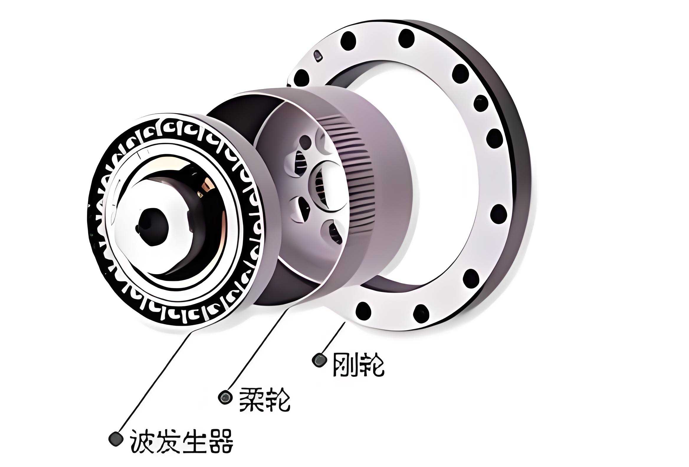
In the field of precision motion control and robotics, strain wave gear drives, also known as harmonic drives, play a pivotal role due to their compact size, high reduction ratios, and minimal backlash. These devices consist of three primary components: a wave generator, a flexspline, and a circular spline. The wave generator induces controlled elastic deformation in the flexspline, enabling meshing with the circular spline to achieve speed reduction. However, a significant challenge in strain wave gear design is the occurrence of tooth tip interference, which can degrade meshing performance, increase wear, reduce accuracy, and compromise load capacity. Traditional design approaches often involve iterative simulation, interference checks, and profile modifications, which are time-consuming and computationally intensive. In this article, I present a novel tooth profile parameter design method that ensures excellent meshing performance by proactively addressing tooth tip interference through a systematic geometric approach. This method eliminates the need for repeated trials and validations, thereby enhancing design efficiency for strain wave gear systems.
The core of the problem lies in the unique kinematics of strain wave gear drives. Unlike conventional gear trains, the meshing process involves continuous elastic deformation of the flexspline, leading to complex relative motions between the flexspline and circular spline teeth. This often results in interference near the tooth tips during engagement and disengagement, particularly in the non-conjugate regions of the profile. To tackle this, we must first understand the motion geometry of the teeth. We establish coordinate systems attached to the circular spline and flexspline, denoted as \( S_C: \{O, \mathbf{e}_{C1}, \mathbf{e}_{C2}\} \) and \( S_f: \{O_f, \mathbf{e}_{f1}, \mathbf{e}_{f2}\} \), respectively. Here, \( O \) is the center of rotation, and \( O_f \) is a point on the neutral layer of the flexspline. The position of a tooth profile point can be described parametrically, and the relative motion is governed by the deformation functions of the flexspline and the rigid-body rotations of the components.
The motion of the flexspline tooth relative to the circular spline tooth can be represented as the transformation between these coordinate systems. Let \( \phi \) be the angular parameter corresponding to the position on the wave generator, and let \( \phi_W \) and \( \phi_F \) be the rotation angles of the wave generator and flexspline output, respectively, relative to the circular spline. For a fixed circular spline, the relationships are derived from the gear ratio. If \( z_F \) and \( z_C \) represent the number of teeth on the flexspline and circular spline, respectively, then:
$$ \phi_W(\phi) = \frac{z_F}{z_C} \phi $$
$$ \phi_F(\phi) = \frac{z_F – z_C}{z_C} \phi $$
The elastic deformation of the flexspline’s neutral layer is described by functions for circumferential deformation \( w(\phi) \), radial deformation \( v(\phi) \), and angular deformation \( \phi_f(\phi) \). Assuming the neutral layer length remains unchanged before and after deformation, we have:
$$ w(\phi) = \rho(\phi) – r_0 $$
$$ v(\phi) = -\int w(\phi) \, d\phi $$
$$ \phi_f(\phi) \approx -\frac{1}{r_0} \left( v(\phi) – \frac{dw}{d\phi} \right) $$
where \( r_0 \) is the undeformed neutral layer radius, and \( \rho(\phi) \) is the radial distance after deformation. For an elliptical wave generator, a common profile, \( \rho(\phi) \) can be expressed as \( \rho(\phi) = r_0 + w_0 \cos(2\phi) \), with \( w_0 \) as the maximum radial deformation. The transformation matrices between coordinate systems are given by rotation matrices \( \mathbf{M}_i \) for \( i = F, W \), and \( \mathbf{M}_{Ff} \) for the deformation:
$$ \mathbf{M}_i = \begin{bmatrix} \cos \phi_i & -\sin \phi_i \\ \sin \phi_i & \cos \phi_i \end{bmatrix}, \quad \mathbf{M}_{Ff} = \begin{bmatrix} \cos \phi_f & -\sin \phi_f \\ \sin \phi_f & \cos \phi_f \end{bmatrix} $$
Thus, the position of a point on the flexspline tooth, such as the tooth tip \( A \), in the circular spline coordinate system is:
$$ \mathbf{R}^C_A = \mathbf{M}_F \left( \mathbf{R}^F_{O_f} + \mathbf{M}_{Ff} \mathbf{R}^f_A \right) $$
where \( \mathbf{R}^F_{O_f} = [v(\phi), r_0 + w(\phi)]^T \). This equation encapsulates the coupled elastic and rigid-body motion, which is fundamental to analyzing meshing in strain wave gear drives.
To design tooth profiles that avoid interference, we focus on the tooth tip motion during disengagement. Let \( \phi_{in} \) and \( \phi_{end} \) denote the angular parameters at the start and end of meshing for a tooth pair. The effective conjugate region corresponds to angles where the tooth profiles theoretically mesh without interference, up to a maximum conjugate angle \( \phi_m \). Beyond \( \phi_m \), the flexspline tooth tip may interfere with the circular spline tooth profile, especially if the circular spline profile is not fully conjugate. The disengagement angle \( \phi_{out} \) is when the flexspline tooth tip clears the circular spline tooth height \( r_{a2} \), determined by solving:
$$ \mathbf{R}^C_A(\phi) \cdot \mathbf{e}_{C2} – r_{a2} = 0 $$
The tooth tip interference criterion is established as follows: interference occurs if the maximum conjugate angle is less than the disengagement angle, i.e.,
$$ \phi_m < \phi_{out} $$
If this criterion holds, we must identify the interference zone. The interference zone \( T \) is defined by critical angles \( \phi_c \) where the flexspline tooth tip trajectory intersects the circular spline tooth profile. We solve for \( \phi \) in:
$$ \mathbf{R}^C_A(\phi) = \mathbf{R}^C_G(s) $$
where \( \mathbf{R}^C_G(s) \) is the circular spline tooth profile parameterized by \( s \). Depending on the number of solutions, we have three cases:
- If no solution exists, interference is absent.
- If one solution \( \phi_{c1} \) exists with \( \phi_m \leq \phi_{c1} < \phi_{out} \), interference persists from \( \phi_{c1} \) to \( \phi_{out} \), so \( T = (\phi_{c1}, \phi_{out}] \).
- If two solutions \( \phi_{c1} \) and \( \phi_{c2} \) exist with \( \phi_m \leq \phi_{c1} < \phi_{c2} \leq \phi_{out} \), interference occurs only between them, so \( T = (\phi_{c1}, \phi_{c2}) \).
Once the interference zone is determined, we generate sample points to guide the tooth profile design. These sample points \( P \) consist of the flexspline tooth tip trajectory points within \( T \) and the effective conjugate points \( Q_1, Q_2, \dots, Q_m \) from the theoretical conjugate curve. That is:
$$ P = \{ \mathbf{R}^C_A(\phi) \mid \phi \in T \} \cup \{ \mathbf{R}^C_{Q_i} \mid i = 1, 2, \dots, m \} $$
By fitting a smooth curve to these sample points, we obtain the circular spline tooth profile that eliminates interference while preserving meshing performance in the conjugate region. This method ensures that the designed profile closely approximates the theoretical conjugate curve, minimizing errors and backlash.
To illustrate this design method, consider a strain wave gear drive with an elliptical wave generator. Assume the flexspline tooth profile parameters are given, as summarized in Table 1. The goal is to design the circular spline tooth profile parameters. The design parameters include module, tooth numbers, addendum coefficients, and deformation characteristics. For instance, let the flexspline have a double-circular-arc tooth profile, which is common in strain wave gear applications for its favorable stress distribution and manufacturing ease.
| Symbol | Description | Value |
|---|---|---|
| \( d_r \) | Flexspline inner diameter (mm) | 60 |
| \( m \) | Module (mm) | 0.3111 |
| \( z_C / z_F \) | Circular spline / flexspline tooth numbers | 202 / 200 |
| \( w^* \) | Deformation coefficient | 1 |
| \( \rho_{a1}^* \) | Addendum radius coefficient for flexspline | 2.0 |
| \( \rho_{f1}^* \) | Dedendum radius coefficient for flexspline | 2.2 |
| \( \zeta_1 \) | Pressure angle at flexspline (°) | 11 |
| \( h_l^* \) | Tooth depth coefficient | 0.74 |
| \( h_{a1}^* \) | Addendum height coefficient for flexspline | 0.8 |
| \( h_{f1}^* \) | Dedendum height coefficient for flexspline | 1.2 |
| \( h_{a2}^* \) | Addendum height coefficient for circular spline | 0.8 |
| \( h_{f2}^* \) | Dedendum height coefficient for circular spline | 1.0 |
The design proceeds step by step. First, we compute the conjugate angles for points on the flexspline tooth profile using the elastic conjugate tooth profile equations based on the instantaneous center method. Due to the double-contact phenomenon in strain wave gear drives, each point on the flexspline may have up to two conjugate angles. For this example, every point exhibits two conjugate instances, as shown in Figure 4(a) of the original text. The theoretical conjugate curves are derived through coordinate transformations, resulting in primary and secondary conjugate curves.
Next, we select effective conjugate points that lie within the circular spline tooth height limits, i.e., between the addendum radius \( r_{a2} \) and dedendum radius \( r_{f2} \). In this case, all points on the primary conjugate curve are valid. Then, we perform an initial curve fitting to these effective conjugate points using a double-circular-arc profile with a common tangent, which yields a preliminary circular spline tooth profile. However, this preliminary profile may still lead to interference, so we apply the interference criterion.
For the given parameters, the maximum conjugate angle \( \phi_m \) is calculated as 52.5918°, and the disengagement angle \( \phi_{out} \) is 62.5198°. Since \( \phi_m < \phi_{out} \), interference is likely. Solving the intersection equation gives two critical angles: \( \phi_{c1} = 52.5918° \) and \( \phi_{c2} = 58° \). Thus, the interference zone is \( T = [52.5918°, 58°] \). We generate sample points \( P \) by including the flexspline tooth tip trajectory points in this zone and the effective conjugate points. A smooth curve is fitted to these sample points, resulting in the final circular spline tooth profile. The profile consists of a convex arc with radius 0.3825 mm and a concave arc with radius 0.6315 mm, ensuring continuity and tangency.
To evaluate the meshing performance of the designed strain wave gear drive, we analyze several key metrics: fitting error, backlash distribution, contact ratio, and maximum engagement depth. These metrics collectively determine the efficiency, accuracy, and durability of the gear system.
The fitting error between the designed circular spline profile and the theoretical conjugate curve indicates how well the profile approximates ideal meshing. For this design, the average fitting error is 0.5 μm, and the maximum fitting error is 0.7 μm, which correspond to 0.0016m and 0.0023m, respectively, where \( m \) is the module. Such small errors demonstrate that the designed profile is extremely close to the theoretical conjugate curve, ensuring near-perfect meshing in the conjugate region. This is crucial for minimizing transmission errors and maximizing torque capacity in strain wave gear drives.
Backlash, the clearance between mating teeth, significantly impacts the dynamic performance and positional accuracy of strain wave gear systems. Excessive backlash can lead to vibration, noise, and reduced precision. Using kinematic simulation, we compute the backlash throughout the meshing cycle. The results show that in the conjugate angle region, backlash remains positive but less than 0.9 μm, with an average of 0.5 μm (0.0016m). Importantly, within the maximum conjugate angle \( \phi_m \), backlash is nearly zero, promoting smooth power transmission. Beyond \( \phi_m \), backlash increases rapidly, reaching 0.0344m at disengagement, which provides ample clearance to avoid tooth tip interference during exit. This backlash distribution is ideal, as it balances minimal play during load-bearing phases with safe disengagement.
The contact ratio \( \varepsilon \) is a measure of how many tooth pairs are in contact simultaneously, directly influencing load distribution and durability. For strain wave gear drives, a higher contact ratio means more teeth share the load, reducing stress on individual teeth. The contact ratio is calculated as:
$$ \varepsilon = \frac{\phi_z}{180^\circ} z_F $$
where \( \phi_z \) is the angular extent of the effective conjugate region. In this example, \( \phi_z = 43.42^\circ \), yielding \( \varepsilon \approx 48 \). This implies that approximately 48 tooth pairs are in contact at any given time under no-load conditions, accounting for about 24% of the total flexspline teeth. Under load, the contact ratio may increase further due to elastic deformation, enhancing the strain wave gear’s load capacity and reliability.
Maximum engagement depth \( h_n \) refers to the depth of tooth interaction along the line of action. A deeper engagement generally allows for higher torque transmission but must be balanced against bending stress and interference risks. The design method here preserves the full addendum heights, so \( h_n \) is not compromised. It can be expressed as:
$$ h_n = (h_{a1}^* + h_{a2}^* – 1 + w^*) m $$
For the given parameters, \( h_n = 1.6m \), which is substantially greater than the module, indicating robust engagement. This is advantageous for strain wave gear drives used in high-torque applications, such as robotic joints or aerospace actuators.
To further generalize the method, we can extend it to other wave generator profiles, such as cam-based or three-lobe designs. The key is to adapt the deformation functions \( w(\phi) \), \( v(\phi) \), and \( \phi_f(\phi) \) accordingly. For instance, for a four-roll wave generator, the neutral layer deformation might be approximated by a Fourier series. The interference criterion and sample point generation remain valid, making this approach versatile for various strain wave gear configurations.
Moreover, the method can be integrated with optimization algorithms to fine-tune tooth profile parameters for specific performance goals. For example, one might minimize backlash variance or maximize contact ratio while constraints on stress and manufacturing tolerances. Table 2 summarizes potential optimization variables and objectives for strain wave gear design.
| Variable | Description | Typical Range |
|---|---|---|
| \( m \) | Module | 0.1–1.0 mm |
| \( w^* \) | Deformation coefficient | 0.8–1.2 |
| \( h_{a1}^*, h_{a2}^* \) | Addendum coefficients | 0.6–1.0 |
| \( \rho_{a1}^*, \rho_{a2}^* \) | Profile radius coefficients | 1.5–3.0 |
| \( \zeta_1, \zeta_2 \) | Pressure angles | 10°–30° |
| Objective | Goal | Metric |
| Minimize backlash | Improve accuracy | Average backlash < 0.001m |
| Maximize contact ratio | Enhance load capacity | \( \varepsilon > 40 \) |
| Minimize stress | Increase fatigue life | Max bending stress < allowable |
| Eliminate interference | Ensure smooth operation | Interference zone \( T = \emptyset \) |
In practice, implementing this design method requires computational tools for solving the geometric equations and performing curve fitting. Software like MATLAB or Python with numerical libraries can automate the process. The steps include: (1) defining the flexspline tooth profile analytically or via discrete points, (2) computing the conjugate curves using the kinematic model, (3) determining the interference zone via root-finding algorithms, (4) generating sample points, and (5) fitting a spline or circular arc profile. This automation reduces human error and accelerates development cycles for strain wave gear drives.
Another aspect to consider is manufacturing tolerances. The designed tooth profiles must be feasible to produce with high precision, as small deviations can affect meshing performance. For strain wave gear drives, processes like hobbing, shaping, or grinding are used. The double-circular-arc profile is particularly amenable to grinding, which can achieve surface finishes suitable for low-friction meshing. Tolerance analysis can be incorporated into the design method by adding safety margins to the interference zone or by simulating profile deviations.
Furthermore, the elastic deformation model used here assumes a thin-walled flexspline with constant thickness. In reality, the flexspline may have variable thickness or complex geometry, such as a cup or pancake design. For more accurate results, finite element analysis (FEA) can be coupled with the geometric model to refine the deformation functions. However, for initial design, the analytical model suffices, as demonstrated by the good meshing performance in the example.
The benefits of this design method extend beyond eliminating interference. By ensuring that the conjugate region is fully utilized, it maximizes the number of teeth in contact, which distributes load more evenly and reduces wear. This is especially important for strain wave gear drives operating in harsh environments or under continuous duty. Additionally, the controlled backlash distribution minimizes dead zones, improving responsiveness in servo applications.
To validate the method experimentally, one could prototype a strain wave gear drive with the designed parameters and measure transmission error, backlash, and efficiency. However, such physical testing is beyond the scope of this article. Instead, we rely on kinematic simulation and error analysis, which are standard practices in gear design. The small fitting errors and favorable backlash distribution provide strong evidence of the method’s effectiveness.
In conclusion, the proposed tooth profile parameter design method for strain wave gear drives offers a systematic approach to ensure excellent meshing performance by proactively addressing tooth tip interference. It leverages motion geometry to establish interference criteria, identify interference zones, and generate guiding sample points for profile design. This eliminates the need for iterative simulations and corrections, saving time and resources. The method has been demonstrated through an example with an elliptical wave generator, resulting in low fitting errors, ideal backlash, high contact ratio, and sufficient engagement depth. These outcomes affirm that the method is both effective and efficient for designing strain wave gear systems that meet demanding performance standards. Future work could explore applications to other gear types or integration with real-time optimization for adaptive designs. As strain wave gear technology advances, such geometric design methods will remain essential for achieving precision and reliability in motion control systems.
Throughout this discussion, the term “strain wave gear” has been emphasized to highlight its relevance in modern engineering. The strain wave gear’s unique principle of operation, relying on elastic deformation, presents both challenges and opportunities for innovation. By adopting advanced design methodologies like the one described here, engineers can harness the full potential of strain wave gear drives in robotics, aerospace, medical devices, and other high-tech fields. The continuous improvement of strain wave gear designs will undoubtedly contribute to more compact, efficient, and reliable mechanical systems worldwide.