
1. Introduction
In my research on mechanical transmission systems, I have focused extensively on the spiral bevel gear because of its outstanding characteristics: large contact ratio, high load-carrying capacity, smooth transmission, low noise, and large transmission ratio. These properties make the spiral bevel gear indispensable in power transmission applications such as automotive differentials, aerospace drive systems, and heavy machinery. The tooth surface of a spiral bevel gear is a complex spatial surface. During traditional cutting, the machine tool must be adjusted repeatedly and the workpiece must be trial-cut. The contact area of the gear pair is then inspected to verify whether the processed spiral bevel gear meets the requirements, and finally the correct machining adjustment parameters are determined. This process not only reduces production efficiency but also increases production cost. With the rapid development of computer technology, digital virtual manufacturing can replace the real trial-cut process to determine the final adjustment parameters for spiral bevel gear machining. This approach can efficiently solve the problems encountered in traditional spiral bevel gear processing.
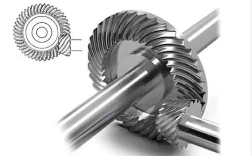
I have established a digital model for the generating method of spiral bevel gear manufacturing, specifically for the pinion. A digital model that can accurately represent the tooth surface of a spiral bevel gear is the foundation of virtual manufacturing. Through in-depth study of the generating principle of spiral bevel gear processing, I discretized the conical surface layers of the gear blank cutting region and the circular layers of the inner and outer cutting surfaces of the tool. I then established a mathematical model for the generating method of spiral bevel gear cutting. After solving this model, processing the discrete points on the tooth surface, and finally connecting these discrete points using a triangular patch method, I obtained a digital model of the spiral bevel gear.
2. Classification and Basic Parameters of Spiral Bevel Gears
The spiral bevel gear can be classified in many ways: by tooth line, by tooth height, and by axis position. I studied these classifications to understand the geometric and manufacturing characteristics of the spiral bevel gear.
2.1 Classification by Tooth Line
According to the tooth line, spiral bevel gear can be divided into three types: circular arc tooth, extended epicycloid tooth, and quasi-involute tooth. The circular arc tooth is generated by a circular face milling cutter using the single indexing method. The extended epicycloid tooth is generated by a face milling cutter using the continuous indexing method. The quasi-involute tooth is generated by a conical hob. Table 1 summarizes these classifications.
| Type | Tooth Line | Generation Method | Typical System |
|---|---|---|---|
| Circular arc | Arc of a circle | Single indexing | Gleason |
| Extended epicycloid | Extended epicycloid | Continuous indexing | Oerlikon, Klingelnberg |
| Quasi-involute | Quasi-involute | Continuous cutting | Rarely used |
2.2 Classification by Tooth Height
According to tooth height, spiral bevel gear can be classified into constant height, tapering height, and double tapering height. In a constant height spiral bevel gear, the root cone angle, pitch cone angle, and face cone angle are equal: \(\beta_1 = \beta_2 = \beta_3\). In a tapering height spiral bevel gear, the tooth height decreases from the large end to the small end, and the face cone angle is larger than the pitch cone angle, which in turn is larger than the root cone angle: \(\beta_3 > \beta_2 > \beta_1\). Double tapering height is a general form, where the root cone vertex lies outside the pitch cone vertex. I treat constant and tapering height as special cases of double tapering height. My research mainly focuses on double tapering height spiral bevel gear.
2.3 Classification by Axis Position
According to axis position, spiral bevel gear pairs can have intersecting axes, non-perpendicular intersecting axes, or offset axes. When the axes are perpendicular and intersecting, the gear pair is a standard spiral bevel gear pair. When the axes are offset, the gear is called a hypoid gear. The offset distance increases the spiral angle and the end face module of the pinion, thereby improving the strength and life of the pinion. However, relative sliding occurs along the tooth length and tooth height directions, causing additional wear.
2.4 Gear Blank Parameters
The spiral bevel gear can be regarded as a straight bevel gear that is divided into infinitely thin slices and then twisted and inclined. Therefore, a straight bevel gear can be considered a special form of spiral bevel gear. The basic parameters of a spiral bevel gear pair include shaft angle, number of teeth, module, hand of spiral, spiral angle, and pressure angle. Table 2 lists the parameters I used in my example.
| Parameter | Symbol | Value |
|---|---|---|
| Number of teeth | \(Z\) | 24 |
| Face width | \(B_F\) | 56 mm |
| Face cone angle | \(\beta_1\) | \(43.08^\circ\) |
| Pitch cone angle | \(\beta_2\) | \(39.37^\circ\) |
| Root cone angle | \(\beta_3\) | \(36.5^\circ\) |
| Spiral angle | \(\beta\) | \(35^\circ\) |
| Hand of spiral | Dir | Right-hand |
| Outer cone distance | \(O_wQ\) | 194.71 mm |
| Inner cone distance | \(O_wP\) | 139.7038 mm |
3. Manufacturing Technology of Spiral Bevel Gears
I studied two main cutting methods for spiral bevel gear: the forming method and the generating method. The forming method uses a formed tool that directly reproduces the tooth profile. The generating method uses a relative motion between the tool and the workpiece to create the tooth surface as an envelope.
3.1 Forming Method
When the pitch cone angle of the large gear is greater than \(70^\circ\) and the transmission ratio is greater than 2.5, the forming method can be used. In this method, the cutter head directly plunges into the blank, and the cradle does not rotate. This greatly simplifies the machine structure and increases productivity by more than 30% compared with the generating method. However, the forming method is mainly suitable for large gears, not for pinions because of their high curvature.
3.2 Generating Method
For pinions and for large gears with pitch cone angles less than \(70^\circ\), the generating method must be used. In the generating method, the cutter head rotates about its own axis and also rotates about the cradle axis, while the workpiece rotates about its own axis according to a certain ratio. The cutter head represents a tooth of an imaginary generating gear, called the cradle gear. The spiral bevel gear tooth surface is generated as the envelope of the cutting edges. Table 3 compares the constant height and tapering height spiral bevel gear in terms of generating method.
| Type | Cutting Method | Efficiency | Strength | Number of Machines | Accuracy |
|---|---|---|---|---|---|
| Constant height | Continuous indexing | High | High | 2 | Lower, cannot be ground |
| Tapering height | Single indexing | Low | Lower | 5 | Higher, can be ground |
3.3 Machine Tool Adjustments
Before cutting a spiral bevel gear, the machine tool must be adjusted according to calculated parameters. The main adjustment parameters are radial cutter position \(S\), cradle angle \(Q\), workpiece mounting angle \(\beta_3\), horizontal wheel position \(X_p\), vertical wheel position \(E_m\), bed position \(X_b\), and roll ratio \(I_{tw}\). Table 4 lists the machine settings I used in my simulation.
| Parameter | Symbol | Value |
|---|---|---|
| Workpiece mounting angle | \(\beta_3\) | \(36.5^\circ\) |
| Horizontal wheel position | \(X_p\) | -9.18 mm |
| Vertical wheel position | \(E_m\) | -3.45 mm |
| Bed position | \(X_b\) | 5.49 mm |
| Radial cutter position | \(S\) | 137.69506 mm |
| Start cradle angle | \(Q_s\) | \(20^\circ\) |
| End cradle angle | \(Q_o\) | \(70^\circ\) |
| Roll ratio | \(I_{tw}\) | 1.48686 |
| Number of discrete points per tooth line | \(n\) | 50 |
4. Coordinate Systems and Transformations
To build the cutting model, I established a machine coordinate system as the absolute reference, with the tool coordinate system and the workpiece coordinate system as local systems. I then derived the transformation algorithms between these systems based on the machine adjustment parameters.
4.1 Machine, Tool, and Workpiece Coordinates
In the machine coordinate system \(O_m – X_m Y_m Z_m\), the tool position is determined by the radial cutter position \(S\) and the cradle angle \(Q\). The horizontal and vertical cutter positions are:
$$
\begin{cases}
H = S \cos Q \\
V = S \sin Q
\end{cases}
$$
The workpiece position is determined by the mounting angle \(\beta_3\), horizontal wheel position \(X_p\), vertical wheel position \(E_m\), and bed position \(X_b\). The transformation matrix from the workpiece coordinate system to the machine coordinate system is:
$$
T_{\text{total}} = T_{X_b} T_{\beta_3} T_{X_p} T_{E_m}
= \begin{bmatrix}
\cos\beta_3 & 0 & \sin\beta_3 & X_p \cos\beta_3 \\
0 & 1 & 0 & E_m \\
-\sin\beta_3 & 0 & \cos\beta_3 & -X_p \sin\beta_3 + X_b \\
0 & 0 & 0 & 1
\end{bmatrix}.
$$
4.2 Geometric Transformations
I used homogeneous coordinates for all transformations. A point \(P(x,y,z)\) is transformed to \(P^*(x^*,y^*,z^*)\) by a matrix multiplication. For example, translation is:
$$
\begin{bmatrix}
x^* \\ y^* \\ z^* \\ 1
\end{bmatrix}
=
\begin{bmatrix}
1 & 0 & 0 & t_x \\
0 & 1 & 0 & t_y \\
0 & 0 & 1 & t_z \\
0 & 0 & 0 & 1
\end{bmatrix}
\begin{bmatrix}
x \\ y \\ z \\ 1
\end{bmatrix}.
$$
Rotation about the \(X\)-axis by angle \(\theta_x\) is:
$$
\begin{bmatrix}
x^* \\ y^* \\ z^* \\ 1
\end{bmatrix}
=
\begin{bmatrix}
1 & 0 & 0 & 0 \\
0 & \cos\theta_x & -\sin\theta_x & 0 \\
0 & \sin\theta_x & \cos\theta_x & 0 \\
0 & 0 & 0 & 1
\end{bmatrix}
\begin{bmatrix}
x \\ y \\ z \\ 1
\end{bmatrix}.
$$
Similar matrices are used for rotations about the \(Y\)- and \(Z\)-axes. I used fixed-coordinate transformations, where each transformation is based on the original coordinate system.
5. Mathematical Modeling of Tool and Gear Blank
5.1 Tool Model Simplification
The disc milling cutter used for spiral bevel gear has many blades. For simulation, I simplified the cutter into a set of conical surfaces and cylindrical surfaces. The simplified tool is defined by eight boundary circles. Table 5 lists the tool parameters I used.
| Parameter | Symbol | Value |
|---|---|---|
| Cutter radius | \(R = D/2\) | 152.4 mm |
| Blade offset | \(W\) | 5.33 mm |
| Tool body base distance | \(K\) | 276 mm |
| Tool body height | \(H\) | 68 mm |
| Tool body thickness | \(H_1\) | 35 mm |
| Blade width | \(B\) | 23.5 mm |
| Mounting hole diameter | \(d\) | 100 mm |
| Outer blade pressure angle | \(a_2\) | \(20.5^\circ\) |
| Inner blade pressure angle | \(a_1\) | \(24.5^\circ\) |
The radii and heights of the eight boundary circles are:
$$
\begin{aligned}
R_0 &= R + \frac{W}{2}, \quad R_7 = R – \frac{W}{2}, \\
R_1 &= R_2 = K + 2B, \\
R_3 &= R_4 = \frac{d}{2}, \\
R_5 &= R_6 = K, \\
H_0 &= H_7 = 0, \\
H_1 &= -\frac{R_1 – R_0}{\tan a_2}, \\
H_2 &= H_3 = -H, \\
H_4 &= H_5 = B – H, \\
H_6 &= -\frac{R_7 – R_6}{\tan a_1}.
\end{aligned}
$$
Any point on a boundary circle \(i\) with radius \(R_i\) and height \(H_i\) is given by:
$$
\begin{cases}
X_t = R_i \cos\theta, \\
Y_t = R_i \sin\theta, \\
Z_t = H_i,
\end{cases}
\quad \theta \in (0, 2\pi).
$$
5.2 Gear Blank Model
The gear blank consists of a tooth part and a base part. I modeled the base part using boundary circles. The radii and heights of the gear blank boundary circles are derived from the gear parameters. For example, the height of the \(N\)-th layer cone is:
$$
H_N = \frac{O_wP – \tan\beta_3 \cdot O_1O_w \cdot \sin\beta_2}{\sin\beta_2 (\cot\beta_2 + \tan\beta_3)},
$$
and the radius of the \(N\)-th boundary circle is:
$$
R_N = -\cot\beta_2 \cdot H_N + \frac{O_wP}{\sin\beta_2}.
$$
Similar equations are used for other boundary circles. The conical surface equation in the workpiece coordinate system is:
$$
X_w – O_wT_N = \cot C_N \sqrt{Y_w^2 + Z_w^2},
$$
where \(C_N\) is the cone angle of the \(N\)-th layer cone.
6. Generating Method Cutting Algorithm
My core contribution is the iterative discrete algorithm for the tool cutting surface. This algorithm is based on the principle that the tool layer circle farthest from the tool top surface is the last one to cut the tooth surface. It avoids the need to consider the mutual influence between successive cutting positions, thus improving efficiency and accuracy.
6.1 Layer Cone Slicing
I divided the gear blank cutting region into \(N\) layer cones. The cone angle of the \(N\)-th layer is:
$$
C_N = C_1 + (N-1) \frac{\theta}{n},
$$
where \(C_1 = \beta_3\) is the root cone angle and \(\theta\) is the angle between the face cone and root cone. The distance from the workpiece origin to the vertex of the \(N\)-th layer cone is:
$$
O_wT_N = -\frac{1}{k_N} \left[ \frac{\tan\beta_3 \tan\beta_1 (O_wO_2 – O_1O_w) – k_N (\tan\beta_1 O_wO_2 – \tan\beta_3 O_1O_w)}{\tan\beta_1 – \tan\beta_3} \right],
$$
where \(k_N = \tan C_N\).
6.2 Iterative Discrete Algorithm for Tool Cutting Surface
For each layer cone, I associated a tool layer circle at a certain height \(Z_N\). The outer and inner radii of the tool layer circle at height \(Z_N\) are:
$$
R_{\text{outer},N} = \frac{D+W}{2} + Z_N \tan a_2,
$$
$$
R_{\text{inner},N} = \frac{D-W}{2} – Z_N \tan a_1.
$$
The tool layer circle equation in the tool coordinate system is:
$$
\begin{cases}
X_t^2 + Y_t^2 = R_N^2, \\
Z_t = -Z_N.
\end{cases}
$$
Because the tooth height of a tapering spiral bevel gear decreases from the large end to the small end, the actual cutting depth \(H_D\) gradually decreases. I set \(H_D = H_2\) initially and iterate until the theoretical layer circle intersects the corresponding layer cone. The flowchart of this algorithm is implemented in my simulation code.
6.3 Intersection Calculation
Transforming the tool layer circle to the machine coordinate system gives:
$$
\begin{cases}
(X_m – H_N)^2 + (Y_m – V_N)^2 = R_N^2, \\
Z_m = -Z_N.
\end{cases}
$$
Transforming the gear blank layer cone to the machine coordinate system gives:
$$
X_m \cos\beta_3 – Z_m \sin\beta_3 + X_b \sin\beta_3 – X_p – O_1T_N = \cot C_N \sqrt{(Y_m – E_m)^2 + (X_m \sin\beta_3 + Z_m \cos\beta_3 – X_b \cos\beta_3)^2}.
$$
Combining these equations yields a quartic equation in \(X_m\):
$$
A X_m^4 + B X_m^3 + C X_m^2 + D X_m + E = 0 \quad (A \neq 0).
$$
I solved this quartic equation using the Ferrari method, which reduces it to a cubic equation and then to a quadratic equation. The roots are checked for validity. A root is valid if it is real and its projection onto the workpiece axis lies within the cutting region.
6.4 Data Point Processing
After obtaining the intersection points, I filtered out invalid points. I used a projection method: for each layer cone, I computed the boundary points \(E\) and \(G\) of the cutting region. A point \(F\) is valid if its projection \(S\) onto the workpiece axis satisfies \(O_wR \leq O_wS \leq O_wT\).
To obtain boundary points, I intersected the line connecting two adjacent valid points with the boundary plane (face cone or back cone). The intersection of a line through \(P(x_1,y_1,z_1)\) and \(Q(x_2,y_2,z_2)\) with a plane \(Ax+By+Cz+D=0\) is:
$$
\begin{cases}
x = \frac{(A x_1 + B y_1 + C z_1 + D)(x_2 – x_1)}{A(x_2 – x_1) + B(y_2 – y_1) + C(z_2 – z_1)} + x_1, \\
y = \frac{(A x_1 + B y_1 + C z_1 + D)(y_2 – y_1)}{A(x_2 – x_1) + B(y_2 – y_1) + C(z_2 – z_1)} + y_1, \\
z = \frac{(A x_1 + B y_1 + C z_1 + D)(z_2 – z_1)}{A(x_2 – x_1) + B(y_2 – y_1) + C(z_2 – z_1)} + z_1.
\end{cases}
$$
Since the number of valid points on each layer may differ, I equalized them by adding midpoints between adjacent points until all layers have the same number of points. This is necessary for triangulation.
To generate the tooth surfaces of adjacent teeth, I rotated the discrete points of the first tooth surface about the workpiece axis. The rotation matrix for the \(N\)-th tooth is:
$$
T_{N-1} =
\begin{bmatrix}
\cos^2\beta_3 + \sin^2\beta_3 \cos\theta_N & \sin\beta_3 \sin\theta_N & -\cos\beta_3 \sin\beta_3 (1-\cos\theta_N) & a_{14} \\
-\sin\beta_3 \sin\theta_N & \cos\theta_N & -\cos\beta_3 \sin\theta_N & a_{24} \\
-\cos\beta_3 \sin\beta_3 (1-\cos\theta_N) & \cos\beta_3 \sin\theta_N & \sin^2\beta_3 + \cos^2\beta_3 \cos\theta_N & a_{34} \\
0 & 0 & 0 & 1
\end{bmatrix},
$$
where \(\theta_N = (N-1)\frac{2\pi}{Z}\), and \(a_{14}, a_{24}, a_{34}\) are translation terms depending on \(X_p\), \(E_m\), and \(X_b\).
6.5 Triangulation
I stored the discrete points in a data structure that includes a 3D pointer array, a triangle vertex list, and a color array. The triangulation connects points from two adjacent layers. For example, given points \(A, B, C, \ldots\) on the first layer and \(a, b, c, \ldots\) on the second layer, I formed triangles \(ABa\), \(Bab\), \(BCb\), \(Cbc\), and so on. For a closed layer, I also connected the last point to the first to close the surface. This produces a smooth and accurate representation of the spiral bevel gear tooth surface.
7. Implementation and Visualization
I implemented the simulation system in Delphi using the GLScene component, which is based on OpenGL. The user interface has four areas: a visualization area, a tool parameter input area, a gear blank parameter input area, and a machine adjustment parameter input area. Three buttons control the display of the tool, the gear blank, and the digital model of the spiral bevel gear.
In GLScene, I placed a camera, a light source, and several dummy cubes to hold the 3D models. The camera is set as the viewer camera, and its target is a dummy cube. This allows the user to rotate, zoom, and pan the model. The tool and gear blank models are generated by connecting the discrete boundary points with triangles. The spiral bevel gear tooth surface is generated by the algorithm described above.
The visualization process includes: calculating the tool and gear blank models, simulating the generating motion, computing the intersection points, filtering and equalizing the points, and finally triangulating the tooth surface. I also implemented the rotation replication to generate all teeth of the spiral bevel gear.
8. Accuracy Verification
To verify the accuracy of my algorithm, I built a parametric model in CATIA using the same control parameters: cradle angle, layer cone angle, cone distance, tool radius, and tool position. I measured the coordinates of the intersection points in CATIA and compared them with my calculated points. Table 6 shows a selection of the comparison. The maximum deviation is on the order of \(0.001\) mm, which confirms the high accuracy of my method.
| Calculated point \((x,y,z)\) | CATIA measured point \((x,y,z)\) | Distance error (mm) |
|---|---|---|
| 196.928802, 26.561129, -18.5 | 196.928795, 26.561118, -18.5 | \(1.30 \times 10^{-5}\) |
| 187.122849, 11.989703, -14.624662 | 187.122379, 11.989522, -14.6247 | \(5.04 \times 10^{-4}\) |
| 185.064865, 6.776661, -9.876662 | 185.064837, 6.776654, -9.87666 | \(2.89 \times 10^{-5}\) |
| 182.824554, 1.638221, -5.122662 | 182.824834, 1.638242, -5.12266 | \(2.81 \times 10^{-4}\) |
| 190.832733, 6.216022, 0 | 190.832727, 6.216012, 0 | \(1.17 \times 10^{-5}\) |
| 180.156357, 18.457762, -18.5 | 180.156436, 18.457762, -18.5 | \(7.90 \times 10^{-5}\) |
| 177.626114, 12.82231, -13.906662 | 177.626214, 12.82242, -13.9067 | \(1.49 \times 10^{-4}\) |
| 174.827072, 7.280586, -9.354662 | 174.827391, 7.280576, -9.35466 | \(3.19 \times 10^{-4}\) |
| 171.794235, 1.866256, -4.838662 | 171.794567, 1.866256, -4.83866 | \(3.32 \times 10^{-4}\) |
| 179.640457, 5.939671, 0 | 179.640347, 5.939662, 0 | \(1.10 \times 10^{-4}\) |
These results demonstrate that my iterative discrete algorithm for the tool cutting surface can produce highly accurate tooth surface points for spiral bevel gear manufacturing.
9. Conclusion
In my research, I developed a digital manufacturing method for spiral bevel gear using the generating method. I established the mathematical models of the tool and gear blank, derived the coordinate transformations, and proposed the iterative discrete algorithm for the tool cutting surface. I implemented the algorithm in Delphi with GLScene visualization and verified the accuracy with CATIA. The main contributions are:
- I determined the gear blank parameters, tool parameters, and machine adjustment parameters for the generating method of spiral bevel gear.
- I established a coordinate system with the machine coordinate as the absolute reference and derived transformation algorithms between tool, workpiece, and machine coordinates.
- I proposed the iterative discrete algorithm for the tool cutting surface, which eliminates the need to consider the mutual influence between successive cutting positions and improves efficiency and accuracy.
- I developed algorithms for filtering valid points, computing boundary points, equalizing the number of points on each layer, and replicating points for adjacent teeth.
- I implemented a visualization system in Delphi and GLScene, and verified the accuracy using CATIA. The deviation is on the order of \(0.001\) mm.
The tooth surface points obtained by my method can be used for tooth contact analysis, error analysis, and strength analysis of spiral bevel gear. In future work, I plan to extend the system to include the forming method for large gears, develop a dynamic simulation of the cutting process, and establish a general interface to export the 3D model to other CAD/CAM software. I also intend to incorporate physical factors such as tool wear and machine deformation to make the simulation more realistic.