
The transmission of motion and power between non-intersecting, non-parallel shafts is a fundamental requirement in advanced mechanical systems such as automotive drivelines, aerospace actuators, and heavy industrial machinery. Hypoid gears are the premier solution for this task, offering the advantages of high load capacity, smooth operation, and the ability to position the pinion axis offset from the gear axis, enabling more compact and optimized drivetrain designs. However, the complex, spatially curved geometry of their tooth surfaces, designed for localized point contact, presents significant challenges in both manufacturing and precise geometrical characterization.
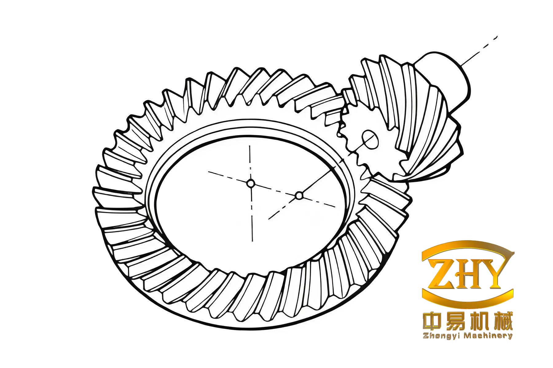
In practical manufacturing of hypoid gears, discrepancies inevitably arise between the theoretical design surface and the physically produced surface due to machine tool errors, setup inaccuracies, tool wear, and heat treatment distortions. To perform accurate contact pattern prediction, transmission error analysis, and ultimately enable error compensation strategies, a high-fidelity digital model of the actual manufactured tooth surface is essential. This process, known as digital tooth surface reconstruction, involves fitting a smooth, continuous mathematical surface to a set of discrete measured or calculated points from the gear tooth. The accuracy and smoothness of this reconstructed surface directly impact the reliability of subsequent simulation and analysis.
Traditional reconstruction methods often utilize simpler interpolation splines, which can suffer from lower accuracy, especially at the surface boundaries, and may not guarantee the required smoothness (continuity of tangency and curvature). This paper addresses this critical issue by proposing and implementing a robust reconstruction algorithm based on Non-Uniform Rational B-Splines (NURBS), enhanced with specific boundary conditions to ensure superior fitting precision at the edges of the hypoid gear tooth surface.
1. Mathematical Foundation: NURBS Curves and Surfaces
Non-Uniform Rational B-Splines (NURBS) have become the industry standard for the representation, design, and data exchange of free-form curves and surfaces. Their power lies in their ability to precisely represent both standard analytic shapes (like conics) and complex free-form geometries using a unified mathematical form. This makes them ideally suited for modeling the sophisticated surfaces of hypoid gears.
1.1 NURBS Curve Formulation
A p-th degree NURBS curve is defined by the following equation:
$$
\mathbf{C}(u) = \frac{\sum_{i=0}^{n} w_i \mathbf{P}_i N_{i,p}(u)}{\sum_{i=0}^{n} w_i N_{i,p}(u)}
$$
Where:
– $\mathbf{P}_i$ are the $(n+1)$ control points forming the control polygon.
– $w_i$ are the corresponding weights, influencing the curve’s proximity to its control points.
– $N_{i,p}(u)$ are the p-th degree B-spline basis functions, defined recursively on a knot vector $\mathbf{U} = \{u_0, u_1, …, u_{m}\}$.
– $u$ is the curve parameter, typically within the interval $[u_p, u_{n+1}]$.
The basis functions are calculated using the Cox-de Boor recursion formula:
$$
\begin{aligned}
N_{i,0}(u) &= \begin{cases}
1 & \text{if } u_i \le u < u_{i+1}\\
0 & \text{otherwise}
\end{cases} \\
N_{i,p}(u) &= \frac{u – u_i}{u_{i+p} – u_i} N_{i,p-1}(u) + \frac{u_{i+p+1} – u}{u_{i+p+1} – u_{i+1}} N_{i+1,p-1}(u)
\end{aligned}
$$
For the reconstruction of hypoid gear tooth surfaces, a cubic degree ($p=3$) is typically chosen as it provides an excellent balance between local shape control, computational efficiency, and smoothness ($C^2$ continuity).
1.2 The Role of End Conditions in Curve Fitting
A crucial step in fitting a NURBS curve to a set of data points (called type points) is determining the end conditions. The standard interpolation problem yields a curve that passes through the points but offers no control over the tangent direction at the start and end. For a closed, smooth profile like a gear tooth curve, this can lead to undesirable “kinks” or inflection points at the boundaries.
To achieve a smoother and more physically accurate reconstruction for hypoid gears, first derivative (tangent vector) end conditions are imposed. This is analogous to fixing the ends of a beam, prescribing the direction of the curve as it enters and leaves the data set. The algorithm enforces:
$$
\mathbf{C}'(u_0) = \mathbf{T}_{start}, \quad \mathbf{C}'(u_{n+1}) = \mathbf{T}_{end}
$$
where $\mathbf{T}_{start}$ and $\mathbf{T}_{end}$ are the prescribed tangent vectors. This constraint is integrated into the system of linear equations solved to find the control points $\mathbf{P}_i$, resulting in a curve that is not only interpolatory but also exhibits superior smoothness at its extremities.
1.3 From Curves to Surfaces: NURBS Surface Formulation
A NURBS surface is a bivariate extension of the NURBS curve, defined as a tensor product of curves in two parametric directions, u and v. A NURBS surface of degree p in the u direction and degree q in the v direction is given by:
$$
\mathbf{S}(u,v) = \frac{\sum_{i=0}^{n} \sum_{j=0}^{m} w_{i,j} \mathbf{P}_{i,j} N_{i,p}(u) N_{j,q}(v)}{\sum_{i=0}^{n} \sum_{j=0}^{m} w_{i,j} N_{i,p}(u) N_{j,q}(v)}
$$
Where:
– $\mathbf{P}_{i,j}$ is a bidirectional $(n+1) \times (m+1)$ net of control points.
– $w_{i,j}$ are the associated weights.
– $N_{i,p}(u)$ and $N_{j,q}(v)$ are the non-rational B-spline basis functions defined on knot vectors $\mathbf{U}$ and $\mathbf{V}$, respectively.
For reconstructing hypoid gear tooth surfaces, a bicubic NURBS surface ($p=3, q=3$) is commonly used. The reconstruction process generally follows these steps:
1. Organize the measured/simulated 3D point cloud from the hypoid gear tooth into a rectangular grid of type points $\mathbf{Q}_{k,l}$.
2. For each row of points (constant v index), fit a NURBS curve with tangent end conditions. This yields a set of control points for each curve.
3. Considering the control points from step 2 as new type points in the perpendicular direction (constant u index), fit another set of NURBS curves to obtain the final two-dimensional grid of surface control points $\mathbf{P}_{i,j}$.
4. The final bicubic NURBS surface $\mathbf{S}(u,v)$ defined by $\mathbf{P}_{i,j}$ provides a smooth, accurate, and computationally efficient digital model of the hypoid gear tooth.
2. Digital Reconstruction Workflow for Hypoid Gears
The proposed methodology for digitally reconstructing hypoid gear tooth surfaces can be systematically broken down into several key stages, from the generation of the reference theoretical surface to the final error assessment.
2.1 Generation of Theoretical Tooth Surface Points
The starting point for validating any reconstruction algorithm is a precise theoretical model. The tooth surface of a hypoid gear is generated via a complex kinematic simulation of the gear manufacturing process (e.g., using a face-milling or face-hobbing method). The mathematical model involves coordinate transformations from the tool coordinate system to the workpiece coordinate system. The surface of the gear (or pinion) can be expressed as a vector function dependent on machine setting parameters and motion parameters:
Gear Tooth Surface Equation:
$$
\mathbf{r}_2 = \mathbf{r}_2(u_2, \theta_2, \phi_2)
$$
Pinion Tooth Surface Equation:
$$
\mathbf{r}_1 = \mathbf{r}_1(u_1, \theta_1, \phi_1)
$$
where $u, \theta$ are parameters defining a point on the cutting tool surface, and $\phi$ represents the rotational motion of the workpiece. By discretizing these parameters over their valid ranges, a dense point cloud representing the flawless, theoretical tooth surface of the hypoid gear is obtained. This cloud serves as the “ground truth” data for the subsequent NURBS reconstruction.
For the purpose of this analysis, a sample hypoid gear set with the following basic design parameters is considered:
| Parameter | Pinion (Concave Side) | Gear (Convex Side) |
|---|---|---|
| Number of Teeth | 10 | 37 |
| Pitch Diameter (mm) | 151.029337 | 372.060000 |
| Mean Pressure Angle (°) | 22.5 | 22.5 |
| Shaft Angle (°) | 90 | 90 |
| Face Width (mm) | 45.52 | 40.00 |
| Spiral Angle (°) | 49.89743 | 37.27946 |
| Hand of Spiral | Left | Right |
Applying the surface equations to this gear set yields a structured grid of points. For instance, a subset of 45 points from the convex surface of the gear is generated as initial type points for reconstruction.
| Point Index | X (mm) | Y (mm) | Z (mm) |
|---|---|---|---|
| 1 | 45.707320 | -3.056529 | -144.053256 |
| 2 | 49.178836 | -4.697160 | -142.813116 |
| 3 | 52.650351 | -6.348760 | -141.552700 |
| 4 | 56.121866 | -8.011764 | -140.271049 |
| 5 | 59.593382 | -9.686633 | -138.967133 |
| … | … | … | … |
| 45 | 76.801596 | 25.892847 | -179.110085 |
2.2 NURBS Curve and Surface Fitting with End Conditions
The core of the proposed algorithm involves fitting a bicubic NURBS surface to the grid of theoretical points, using the enhanced boundary condition.
Step 1: Boundary Condition Specification. For each row and column of points in the grid, the tangent vectors at the start and end of the curve are calculated or estimated (e.g., using a finite difference method based on neighboring points). These vectors, $\mathbf{T}_{start}$ and $\mathbf{T}_{end}$, are then fixed as constraints for the curve fitting process for all hypoid gear profile curves.
Step 2: Parameterization and Knot Vector Generation. The chord length parameterization method is used to assign parameter values to the type points, as it approximates the arc length and generally leads to good shape fidelity. For cubic interpolation of $(n+1)$ points with clamped end conditions (multiplicity 4 at ends), the knot vector $\mathbf{U}$ is constructed accordingly.
Step 3: Control Point and Weight Calculation. For each set of points (e.g., a row along the tooth profile), a system of linear equations is built incorporating the point interpolation constraints and the fixed tangent end conditions. Solving this system yields the control points $\mathbf{P}_i$ for that NURBS curve. The weights $w_i$ are typically set to 1 for standard interpolation, but can be adjusted for specific conic sections if needed. This process is repeated for all rows.
Step 4: Surface Construction. The control points obtained from the row-wise curve fits are treated as new type points for column-wise fitting. The same cubic NURBS interpolation with end conditions is performed in this orthogonal direction. The final output is the complete net of control points $\mathbf{P}_{i,j}$ and the associated knot vectors $\mathbf{U}$ and $\mathbf{V}$ defining the bicubic NURBS surface $\mathbf{S}(u,v)$. This surface can be exported in standard formats like IGES for use in CAD/CAM/CAE systems.
3. Error Analysis and Validation
To quantitatively evaluate the precision of the proposed NURBS reconstruction method for hypoid gears, an error analysis is performed by comparing the reconstructed surface against the original theoretical point cloud.
3.1 Absolute Error Calculation Method
The absolute error at a given point on the reconstructed hypoid gear surface is defined as the shortest distance between that point and the theoretical surface. A practical computational method involves the following: For a reconstructed surface point $\mathbf{P}_r(x_r, y_r, z_r)$, find the corresponding theoretical surface point $\mathbf{P}_t(x_t, y_t, z_t)$ that shares the same $(x, y)$ coordinates (projection onto a plane). The theoretical $z_t$ value for $(x_r, y_r)$ is calculated from the precise mathematical surface equations $\mathbf{r}(u, \theta, \phi)$. The absolute error $\Delta Z$ is then:
$$
\Delta Z = | z_t – z_r |
$$
This error metric is calculated for a representative sample of points across the reconstructed hypoid gear tooth surface.
3.2 Error Results and Discussion
The error analysis demonstrates the high accuracy achieved by the NURBS reconstruction with end tangent conditions. The following table shows the calculated absolute errors for a sample curve (first row of the grid) on the gear’s convex surface:
| Theoretical Point (x, y) mm | Theoretical z_t (mm) | Reconstructed z_r (mm) | Absolute Error ΔZ (μm) |
|---|---|---|---|
| (45.978512, -9.003078) | -143.865438 | -143.865525 | 0.087 |
| (49.530631, -10.485643) | -142.670546 | -142.670467 | 0.079 |
| (51.010063, -11.479134) | -141.721745 | -141.721699 | 0.046 |
| (53.683824, -12.461125) | -140.868639 | -140.868549 | 0.090 |
| (56.702335, -13.613631) | -139.684491 | -139.684427 | 0.064 |
The results consistently show that the absolute error for the reconstructed hypoid gear surface using the proposed method is less than 0.1 micrometers (μm). This exceptional level of precision is critical for high-fidelity contact stress analysis and transmission error calculation. Furthermore, visual inspection and curvature analysis confirm that the reconstructed surface exhibits superior smoothness, particularly at the boundaries (toe, heel, tip, and root), eliminating the kinks or flat spots that can occur with free-end condition interpolation. This smoothness is vital for simulating realistic contact conditions under load for hypoid gears.
4. Conclusion
This work presents a comprehensive methodology for the high-precision digital reconstruction of hypoid gear tooth surfaces. By leveraging the powerful mathematical framework of Non-Uniform Rational B-Splines (NURBS) and augmenting the standard interpolation algorithm with first-derivative (tangent vector) end conditions, significant improvements in both accuracy and smoothness are achieved.
The key contributions and findings are summarized as follows:
- Enhanced Boundary Fidelity: The imposition of tangent end conditions during the NURBS curve fitting stage ensures that the reconstructed curves, which form the building blocks of the surface, are exceptionally smooth from start to finish. This directly translates to a reconstructed hypoid gear tooth surface with superior continuity at its boundaries (toe, heel, tip, root), areas that are critical for accurate edge contact prediction.
- Sub-Micron Reconstruction Accuracy: The proposed algorithm achieves an absolute fitting error of less than 0.1 μm when reconstructing the theoretical surface of a hypoid gear. This level of precision is superior to methods that do not enforce such boundary conditions and is fully sufficient for advanced gear metrology, digital twin creation, and closed-loop manufacturing error compensation.
- Systematic Workflow: A clear, step-by-step workflow is established, from the generation of reference data via gear theory equations, through the parameterization and constrained curve fitting, to the final tensor-product surface construction. This workflow is automatable and applicable to both simulated theoretical surfaces and point clouds obtained from physical coordinate measurement machines (CMM) for real hypoid gears.
The developed digital reconstruction model provides an essential tool for the modern design and analysis of hypoid gears. It enables accurate virtual tooth contact analysis (TCA) and loaded tooth contact analysis (LTCA) based on as-manufactured geometry, facilitates root cause analysis of manufacturing errors, and paves the way for intelligent machining correction strategies. Future work may focus on applying this reconstruction technique to measured point clouds from physical hypoid gear specimens, integrating it with on-machine measurement systems, and extending the optimization to minimize deviations from a desired contact pattern.