
Straight bevel gears represent a geometrically simple, easily manufacturable, and economical type of bevel gear. In theory, the line of contact for these gears should extend across the entire face width. However, in practice, machining errors of the gears and their housing, assembly inaccuracies, and deflections under load can cause a shift in meshing position. This often leads to localized contact concentrated at either the toe or the heel of the tooth, resulting in significant stress concentration at the ends of the tooth flank. This stress concentration is a primary cause of premature gear failure. Furthermore, such misalignment contributes to less smooth operation and increased noise generation. Consequently, conventional straight bevel gears are typically limited to applications with low peripheral speeds (less than 5 m/s) and moderate power transmission.
As demands for higher speeds and heavier loads in gear drives, including bevel gear sets, continue to grow, standard straight bevel gears often fall short. In response, gear experts have proposed modifying the tooth trace—the line along the face width—from a straight line to a slightly crowned, or “drum-shaped,” profile. This deliberate crowning allows for precise control over the contact pattern’s location and size, ensuring a defined area of localized contact along the tooth length. The key benefit is that even in the presence of minor manufacturing tolerances, heat treatment distortions, assembly errors, or load-induced deflections, the contact area remains within the central portion of the tooth, preventing detrimental end-contact and the associated stress peaks.
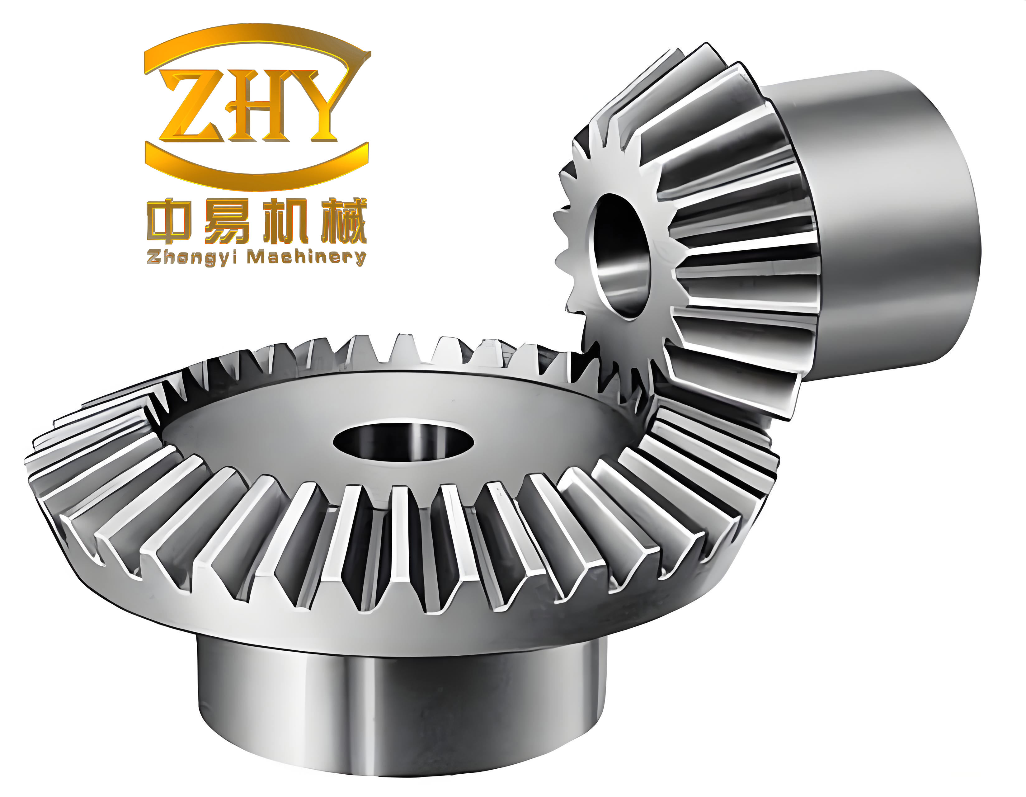
In other words, drum-shaped straight bevel gears exhibit reduced sensitivity to errors and deflections. This significantly enhances transmission quality, improves gear life, and effectively broadens the application range for this gear type. While spiral bevel gears or hypoid gears can be selected for high-power, high-speed applications, they require specialized, costly manufacturing equipment and involve longer production cycles. Therefore, in many scenarios, employing drum-shaped straight bevel gears offers a more convenient and economical solution without sacrificing performance.
Key Factors and Methodology for Determining Crown Amount
Factors Influencing Crown Amount Selection
The primary objective of crowning a straight bevel gear tooth is to establish a correct, controlled contact pattern during operation and to avoid edge contact. Therefore, the amount of crown, or “drum shape,” is a critical parameter that must be carefully chosen. An excessive crown reduces the effective contact area, leading to non-uniform load distribution and increased localized contact stress, which can paradoxically shorten gear life. Conversely, insufficient crown fails to provide the intended benefits of error compensation. Determining the optimal crown amount requires a holistic consideration of the following influencing factors:
- Manufacturing precision of the gears and the gearbox housing, along with the quality of assembly.
- Material properties and heat treatment of the gears, which must ensure adequate strength and durability.
- System deformations, including elastic deflections (tooth contact deformation, bending, and torsional wind-up of the shafts) and systemic variations (bearing clearances, oil film thickness).
- Geometric parameters of the gear, specifically the face width and module.
Determining the Crown Amount
Theoretically, calculating the optimal crown amount should involve all the aforementioned factors. However, due to the complexity and interdependence of these variables, a comprehensive analytical method is not yet fully established for straight bevel gears. In practical engineering applications, an empirical selection approach is widely adopted. Based on experience, the recommended crowning amount $\Delta S$ along the tooth trace typically falls within the following ranges:
- $0.03 \text{ mm}$ to $0.05 \text{ mm}$ (absolute value)
- Or, $0.004m$ to $0.005m$, where $m$ is the module of the gear.
The table below summarizes these empirical guidelines and their typical application context.
| Type of Modification | Recommended Crown Amount ($\Delta S$) | Typical Application Context | Notes |
|---|---|---|---|
| Trace Crowning (Drum Shape) | $0.03$ mm to $0.05$ mm | General purpose, moderate precision gears. | Absolute value, independent of size. |
| Trace Crowning (Drum Shape) | $0.004m$ to $0.005m$ | Scaled approach for gears of varying size. | Proportional to the module $m$. |
Machining Drum-Shaped Teeth on a Conventional Bevel Gear Generator
Introduction to the Tracer Modification Attachment
Machining drum-shaped teeth on straight bevel gears is typically performed on specialized machines, such as the Gleason No. 24A bevel gear generator, which offers high quality and precise control over the crown amount. However, in the absence of such dedicated equipment, it is feasible to retrofit a standard machine with an add-on attachment. This section explores a method for machining crowned teeth on a Y2380 bevel gear planer by integrating a custom-designed tracer modification device.
The fundamental principle involves superimposing a small, controlled oscillatory motion onto the linear reciprocation of the cutting tool. On a standard Y2380 planer, the tool slide is constrained to move in a straight line during the cutting stroke when producing conventional straight teeth. The modification device replaces this rigid constraint with a follower system. A template (tracer) with a specific profile is used. As the machine cycle progresses, a roller follower traces this template profile. This motion is translated via a lever mechanism to induce a slight rocking motion in the tool slide around its pivot axis.
This rocking motion provides an additional displacement component to the cutting tool in the direction of the tooth height. Consequently, the path traced by any point on the cutting edge becomes a composite of the primary linear stroke and this secondary arcuate motion, resulting in a crowned tooth flank. It is important to note that with this kinematic principle, the root fillet of the gear tooth is also machined to a curved profile. For a typical crown amount $\Delta S = 0.05$ mm, the maximum additional displacement of the tool in the height direction, $\Delta H$, can be calculated. A minor increase in the tooth depth at both the toe and heel can compensate for this without affecting the working clearance. The position of the crown’s apex (the highest point of the tooth) can be adjusted by altering the fixed position of the template or by designing its curve accordingly.
Design and Calculation of the Tracer Curve
The profile of the tracer directly defines the crown shape on the straight bevel gear tooth. Several curve types can be employed depending on the desired contact pattern under load:
- Single Circular Arc: Places the contact at the center of the face width. Easiest to calculate and manufacture.
- Parabolic Curve: Offers a more gradual transition and can be designed for a specific contact zone.
- Three-Segment Curve: A compound curve offering high flexibility for optimizing contact under complex load conditions.
Based on practical experience, contact patterns located towards the toe (approximately at one-third of the face width from the small end) often run-in more effectively and result in quieter operation compared to a perfectly centered pattern. Therefore, using two parabolic segments to approximate the desired crowned shape can be advantageous over a single circular arc. The following presents the calculation for a two-parabola tracer curve designed to provide a crown amount $\Delta S$ with its apex at a specified point along the face width. The calculation framework establishes the equations for the two parabolic segments $L_1$ and $L_2$ that together form a smooth, continuous crown curve.
Let us define the coordinate system for the tracer curve. The x-axis represents the normalized position along the face width of the straight bevel gear (from toe to heel), and the y-axis represents the corresponding displacement imparted to the tool. We aim for a total crown height of $\Delta S$. For a face width $B$, we define key points. Let the apex of the crown (point of maximum y-value, $R$) be located at $x = -\frac{B}{6}$ (placing it towards the toe). We define the crown amount such that at the endpoints (toe at $x = -\frac{B}{2}$ and heel at $x = +\frac{B}{2}$), the y-value is $R – \frac{\Delta S}{2}$. We construct the curve from two parabolic segments $L_1$ and $L_2$ meeting smoothly at the apex $M_2\left(-\frac{B}{6}, R\right)$.
Segment L1 (from near toe to apex): This parabola passes through point $M_1\left(-\frac{B}{2}, R – \frac{\Delta S}{2}\right)$, the apex $M_2\left(-\frac{B}{6}, R\right)$, and a symmetry-mirrored point $M_3\left(+\frac{B}{6}, R – \frac{\Delta S}{2}\right)$ (note: this point ensures the left parabola’s shape but is not its right endpoint). Its general form is $y = f_1(x) = a_1x^2 + b_1x + c_1$. Substituting the coordinates of $M_1$, $M_2$, and $M_3$ yields the following system of equations:
$$
\begin{cases}
R – \frac{\Delta S}{2} = a_1\left(-\frac{B}{2}\right)^2 + b_1\left(-\frac{B}{2}\right) + c_1 = \frac{B^2}{4}a_1 – \frac{B}{2}b_1 + c_1 \\
R = a_1\left(-\frac{B}{6}\right)^2 + b_1\left(-\frac{B}{6}\right) + c_1 = \frac{B^2}{36}a_1 – \frac{B}{6}b_1 + c_1 \\
R – \frac{\Delta S}{2} = a_1\left(+\frac{B}{6}\right)^2 + b_1\left(+\frac{B}{6}\right) + c_1 = \frac{B^2}{36}a_1 + \frac{B}{6}b_1 + c_1
\end{cases}
$$
Subtracting the third equation from the first eliminates $a_1$ and $c_1$ and allows solving for $b_1$:
$$
\left( \frac{B^2}{4}a_1 – \frac{B}{2}b_1 + c_1 \right) – \left( \frac{B^2}{36}a_1 + \frac{B}{6}b_1 + c_1 \right) = 0
$$
$$
\left( \frac{9B^2}{36}a_1 – \frac{B^2}{36}a_1 \right) + \left( -\frac{3B}{6}b_1 – \frac{B}{6}b_1 \right) = 0
$$
$$
\frac{8B^2}{36}a_1 – \frac{4B}{6}b_1 = 0 \quad \Rightarrow \quad \frac{2B^2}{9}a_1 = \frac{2B}{3}b_1 \quad \Rightarrow \quad b_1 = \frac{B}{3}a_1
$$
Subtracting the second equation from the third (or first) helps find $a_1$. Subtract the second from the third:
$$
\left( R – \frac{\Delta S}{2} \right) – R = \left( \frac{B^2}{36}a_1 + \frac{B}{6}b_1 + c_1 \right) – \left( \frac{B^2}{36}a_1 – \frac{B}{6}b_1 + c_1 \right)
$$
$$
-\frac{\Delta S}{2} = \frac{B}{3}b_1
$$
Substitute $b_1 = \frac{B}{3}a_1$:
$$
-\frac{\Delta S}{2} = \frac{B}{3} \cdot \frac{B}{3}a_1 = \frac{B^2}{9}a_1
$$
Therefore:
$$
a_1 = -\frac{9\Delta S}{2B^2}
$$
Then:
$$
b_1 = \frac{B}{3} \cdot \left(-\frac{9\Delta S}{2B^2}\right) = -\frac{3\Delta S}{2B}
$$
Now solve for $c_1$ using the second equation $R = \frac{B^2}{36}a_1 – \frac{B}{6}b_1 + c_1$:
$$
R = \frac{B^2}{36}\left(-\frac{9\Delta S}{2B^2}\right) – \frac{B}{6}\left(-\frac{3\Delta S}{2B}\right) + c_1
$$
$$
R = -\frac{\Delta S}{8} + \frac{\Delta S}{4} + c_1 = \frac{\Delta S}{8} + c_1
$$
$$
c_1 = R – \frac{\Delta S}{8}
$$
Thus, the equation for segment $L_1$ is:
$$
\boxed{f_1(x) = -\frac{9\Delta S}{2B^2}x^2 – \frac{3\Delta S}{2B}x + \left(R – \frac{\Delta S}{8}\right)}
$$
Valid for $-\frac{B}{2} \le x \le -\frac{B}{6}$.
Segment L2 (from apex to heel): This parabola passes through the apex $M_2\left(-\frac{B}{6}, R\right)$, a point $M_4\left(-\frac{5B}{6}, R – \frac{\Delta S}{2}\right)$ (mirroring the start of the full curve), and the heel endpoint $M_5\left(+\frac{B}{2}, R – \frac{\Delta S}{2}\right)$. Its form is $y = f_2(x) = a_2x^2 + b_2x + c_2$. Substituting the points:
$$
\begin{cases}
R – \frac{\Delta S}{2} = a_2\left(-\frac{5B}{6}\right)^2 + b_2\left(-\frac{5B}{6}\right) + c_2 = \frac{25B^2}{36}a_2 – \frac{5B}{6}b_2 + c_2 \\
R = a_2\left(-\frac{B}{6}\right)^2 + b_2\left(-\frac{B}{6}\right) + c_2 = \frac{B^2}{36}a_2 – \frac{B}{6}b_2 + c_2 \\
R – \frac{\Delta S}{2} = a_2\left(+\frac{B}{2}\right)^2 + b_2\left(+\frac{B}{2}\right) + c_2 = \frac{B^2}{4}a_2 + \frac{B}{2}b_2 + c_2
\end{cases}
$$
Following a similar solving process (subtracting equations to eliminate variables), we find the coefficients for $L_2$. Subtract the first equation from the third to eliminate $c_2$ and find a relation between $a_2$ and $b_2$:
$$
\left( \frac{B^2}{4}a_2 + \frac{B}{2}b_2 + c_2 \right) – \left( \frac{25B^2}{36}a_2 – \frac{5B}{6}b_2 + c_2 \right) = 0
$$
$$
\left( \frac{9B^2}{36}a_2 – \frac{25B^2}{36}a_2 \right) + \left( \frac{3B}{6}b_2 + \frac{5B}{6}b_2 \right) = 0
$$
$$
-\frac{16B^2}{36}a_2 + \frac{8B}{6}b_2 = 0 \quad \Rightarrow \quad -\frac{4B^2}{9}a_2 + \frac{4B}{3}b_2 = 0 \quad \Rightarrow \quad b_2 = \frac{B}{3}a_2
$$
Now subtract the second equation from the first:
$$
\left( R – \frac{\Delta S}{2} \right) – R = \left( \frac{25B^2}{36}a_2 – \frac{5B}{6}b_2 + c_2 \right) – \left( \frac{B^2}{36}a_2 – \frac{B}{6}b_2 + c_2 \right)
$$
$$
-\frac{\Delta S}{2} = \left( \frac{24B^2}{36}a_2 \right) – \left( \frac{4B}{6}b_2 \right) = \frac{2B^2}{3}a_2 – \frac{2B}{3}b_2
$$
Substitute $b_2 = \frac{B}{3}a_2$:
$$
-\frac{\Delta S}{2} = \frac{2B^2}{3}a_2 – \frac{2B}{3} \cdot \frac{B}{3}a_2 = \frac{2B^2}{3}a_2 – \frac{2B^2}{9}a_2 = \frac{4B^2}{9}a_2
$$
Therefore:
$$
a_2 = -\frac{9\Delta S}{8B^2}
$$
Then:
$$
b_2 = \frac{B}{3} \cdot \left(-\frac{9\Delta S}{8B^2}\right) = -\frac{3\Delta S}{8B}
$$
Solve for $c_2$ using the second equation $R = \frac{B^2}{36}a_2 – \frac{B}{6}b_2 + c_2$:
$$
R = \frac{B^2}{36}\left(-\frac{9\Delta S}{8B^2}\right) – \frac{B}{6}\left(-\frac{3\Delta S}{8B}\right) + c_2
$$
$$
R = -\frac{\Delta S}{32} + \frac{\Delta S}{16} + c_2 = \frac{\Delta S}{32} + c_2
$$
$$
c_2 = R – \frac{\Delta S}{32}
$$
Thus, the equation for segment $L_2$ is:
$$
\boxed{f_2(x) = -\frac{9\Delta S}{8B^2}x^2 – \frac{3\Delta S}{8B}x + \left(R – \frac{\Delta S}{32}\right)}
$$
Valid for $-\frac{B}{6} \le x \le +\frac{B}{2}$.
To ensure a smooth transition (equal slope) at the junction $x = -\frac{B}{6}$, we check the derivatives:
$$
f_1′(x) = -\frac{9\Delta S}{B^2}x – \frac{3\Delta S}{2B} \quad \Rightarrow \quad f_1’\left(-\frac{B}{6}\right) = -\frac{9\Delta S}{B^2}\left(-\frac{B}{6}\right) – \frac{3\Delta S}{2B} = \frac{3\Delta S}{2B} – \frac{3\Delta S}{2B} = 0
$$
$$
f_2′(x) = -\frac{9\Delta S}{4B^2}x – \frac{3\Delta S}{8B} \quad \Rightarrow \quad f_2’\left(-\frac{B}{6}\right) = -\frac{9\Delta S}{4B^2}\left(-\frac{B}{6}\right) – \frac{3\Delta S}{8B} = \frac{3\Delta S}{8B} – \frac{3\Delta S}{8B} = 0
$$
The slopes match at the apex, confirming a smooth curve. The total crown amount $\Delta S$ is the difference in $y$ between the apex and the endpoints:
$$
\Delta S = R – \left(R – \frac{\Delta S}{2}\right) = \frac{\Delta S}{2} \times 2 = \Delta S
$$
This validates the design. The value of $R$, the apex height, is determined by setting the endpoint condition in either $f_1$ or $f_2$. Using $f_1(-\frac{B}{2}) = R – \frac{\Delta S}{2}$ confirms consistency.
Proposed Methods for Enhancing the Quality of Crowned Straight Bevel Gears
The kinematic principle of the tracer attachment described, while functional, presents a theoretical limitation. The crowning is achieved by inducing a tool swing that adds motion primarily in the tooth height direction. This results in a curved root fillet and may not produce the ideal crowned flank topography. A more refined approach would involve generating the crown by imparting a controlled, subtle motion to the cutting tool in the direction of the tooth thickness (i.e., tangential to the pitch cone). This method would theoretically produce a more ideal localized contact pattern on the flanks of the straight bevel gears while maintaining a straighter root fillet. Developing such a mechanism warrants further research.
Furthermore, these crowned straight bevel gears are frequently case-hardened (e.g., carburized and quenched) to achieve high surface durability. Heat treatment inevitably introduces distortions, and the shift in machining and assembly datums before and after hardening can degrade precision. A gear pair with excellent pre-heat-treatment contact may exhibit significant pattern shift and reduced accuracy post-hardening. To counter this, a two-stage manufacturing strategy can be employed:
- Pre-Grind/Pre-Finish: Machine the gear teeth before case hardening, but leave a small, consistent stock allowance on the flanks.
- Post-Hardening Finishing: After hardening, precision-grind all critical locating surfaces and assembly datums (e.g., bore, back face). Using these newly established high-precision datums, perform a final hard-finishing operation on the crowned tooth flanks. For very hard materials, this could be a specialized grinding or hard-skiving process tailored for the crowned profile.
This process chain significantly enhances the final accuracy, stability of the contact pattern, and overall transmission quality of the straight bevel gears.
The table below contrasts the discussed machining and finishing approaches.
| Method | Principle | Advantages | Limitations/Challenges | Best For |
|---|---|---|---|---|
| Tracer Attachment on Planer | Tool swing adds height-direction motion. | Adaptable to standard machines; cost-effective for prototypes/small batches. | Curved root fillet; crown shape kinematically linked to tool path; limited precision. | Soft-state pre-machining, low-volume production. |
| Dedicated Crown-Generating Machine | Integrated CNC or mechanical crowning capability. | High precision and repeatability; excellent control over crown amount and location. | High capital investment; requires specialized equipment. | Medium to high-volume production of quality gears. |
| Axial Tool Motion Concept | Tool motion in tooth thickness direction. | Potentially more ideal flank topography; straighter root fillet. | Requires development of new machine kinematics or attachments. | Future high-performance applications (theoretical). |
| Post-Hardening Finishing (Grinding/Skiving) | Material removal after heat treatment on re-established datums. | Compensates for heat treat distortion; achieves highest final accuracy and surface quality. | Requires hard-finishing capability; additional process step increases cost. | High-performance, hardened straight bevel gears for critical applications. |
Conclusion
The manufacturing of drum-shaped, or crowned, straight bevel gears is an important technological advancement. It directly addresses the limitations of traditional straight-tooth designs by mitigating sensitivity to errors and misalignments. This leads to expanded application ranges, improved service life, and reduced operational noise for straight bevel gear drives. While specialized machines offer optimal results, the exploration of retrofit solutions on conventional planers demonstrates the underlying principles and provides a viable path for implementation where dedicated resources are unavailable.
The design of the crowning curve, particularly using composed parabolic segments, allows for targeted contact pattern placement, optimizing performance based on empirical knowledge of straight bevel gear behavior. Looking forward, the development of more sophisticated crowning kinematics and the integration of robust post-hardening finishing processes are key areas for further research. These advancements will continue to push the boundaries of performance, reliability, and economic viability for straight bevel gears in modern mechanical power transmission systems.