
In modern mechanical and electromechanical systems, screw gears, such as worm drives, play a crucial role in transmitting motion and torque with high reduction ratios and compact design. The integration of electromagnetic principles into screw gear systems has led to the development of electromechanical integrated electromagnetic worm drives, which offer advantages like non-contact operation, reduced friction, and self-protection against overloads. However, these systems exhibit complex dynamic behaviors due to time-varying electromagnetic meshing stiffness, resulting from periodic changes in the number of meshing magnetic poles. This time-varying stiffness introduces parametric excitation, making the system susceptible to parameter vibrations, including free vibrations, main resonance, and combination resonance. In this article, I explore the parameter vibration response of such screw gear systems, focusing on deriving analytical solutions, analyzing resonance phenomena, and presenting results through mathematical formulations, tables, and computational insights. The goal is to provide a comprehensive understanding of the dynamics that can inform the design and optimization of screw gear systems in applications like aerospace, automotive, and robotics.
The core of the analysis lies in modeling the electromechanical integrated screw gear system as a parameter vibration system. The screw gear mechanism typically consists of an electromagnetic worm (screw) with coiled windings and a worm wheel with permanent magnets. When alternating current flows through the worm coils, a rotating magnetic field is generated, driving the worm wheel via magnetic forces. This setup eliminates direct mechanical contact, akin to traditional screw gears, but introduces electromagnetic coupling that varies with meshing conditions. The periodic engagement and disengagement of magnetic poles cause the electromagnetic meshing stiffness to fluctuate over time, leading to a linear time-varying differential equation that governs the system’s dynamics. I begin by deriving the expression for this time-varying stiffness in Fourier series form, which serves as the foundation for the vibration analysis.
Consider a screw gear system where the worm wheel has z permanent magnet teeth, and the wrap angle between the worm and wheel is φ_v. The meshing stiffness varies between one and two pairs of teeth engaging, similar to the contact patterns in mechanical screw gears. Let T_p be the meshing period, given by T_p = 2π / (z ω_p), where ω_p is the rotational angular velocity of the worm wheel. The contact ratio ε_p is defined as the weighted average of engagement pairs. For instance, with one pair engaging for a fraction of the period and two pairs for the remainder, the stiffness function k(t) can be expressed as a piecewise function. Based on electromagnetic theory, the stiffness for one pair engagement, k_{p1}, is derived from the magnetic energy and inductance between the worm coils and wheel teeth. A general form is:
$$ k_{p1} = K \frac{I_s^2 z^2 L_1}{2r^2} \cos(z \theta + \phi_v / (3n_1 p)) \bigg|_{\theta=\theta_0} $$
where K is a constant depending on the wrap angle, I_s is the current in the worm coils, L_1 is the average inductance, r is the wheel radius, θ is the relative rotation angle, θ_0 is the static angle, n_1 is the number of current phases, and p is the pole number. The time-varying stiffness k(t) alternates between k_{p1} and k_{p2} = 2k_{p1} over the meshing period. Since k(t) is an even periodic function, it can be expanded into a complex Fourier series:
$$ k(t) = \sum_{n=-\infty}^{+\infty} k_n e^{i(2n\pi t / T_p)} $$
The Fourier coefficients k_n are calculated by integrating over one period. The average stiffness \bar{k} is the DC component k_0, and the time-varying part Δk(t) represents the oscillatory components. For the screw gear system with z=8 and a wrap angle of 80°, the coefficients simplify to:
$$ k_0 = \frac{16}{9} k_{p1}, \quad k_n = -\frac{k_{p1}}{n\pi} \sin\left(\frac{2n\pi}{9}\right) \text{ for } n \neq 0 $$
Thus, the stiffness function becomes:
$$ k(t) = \bar{k} + \Delta k(t) = k_0 – \frac{k_{p1}}{\pi} \sum_{n=1}^{\infty} \frac{\sin(2n\pi/9)}{n} \left(e^{i n \omega_p t} + e^{-i n \omega_p t}\right) $$
This expression highlights the parametric nature of the system, where the stiffness varies harmonically at multiples of the meshing frequency ω_p. To analyze the vibration response, I use a lumped-parameter model for the screw gear system. The wheel is modeled as a mass m with torsional displacement x (linearized as linear displacement at radius r), damping coefficient c, and the time-varying stiffness k(t). The equation of motion, considering an external torque fluctuation ΔT cos ω t on the wheel, is:
$$ m\ddot{x} + c\dot{x} + k(t)x = \frac{\Delta T \cos \omega t}{r} $$
Substituting the stiffness expression and normalizing, I obtain a parameter vibration equation:
$$ \ddot{x} + 2\zeta_0 \omega_0 \dot{x} + \omega_0^2 \left[1 – \varepsilon \sum_{n=1}^{\infty} b_n \left(e^{i n \omega_p t} + e^{-i n \omega_p t}\right)\right] x = \frac{T’}{m r} \cos \omega t $$
where ω_0 = \sqrt{\bar{k}/m} is the natural frequency, ζ_0 = c/(2ω_0 m) is the damping ratio, ε = a_1 is a small parameter with a_n = k_{p1} \sin(2n\pi/9)/(n\pi \omega_0^2), b_n = a_n/a_1, and T’ is an equivalent load amplitude. This equation forms the basis for investigating free and forced vibrations in screw gear systems.
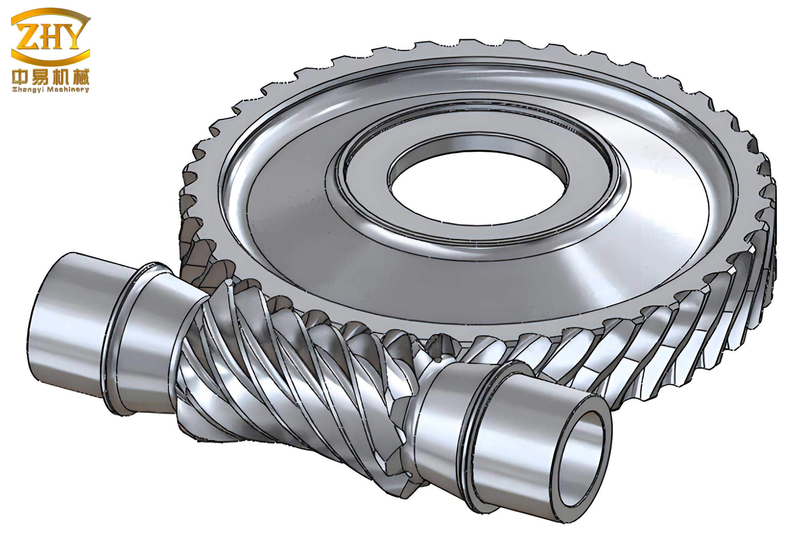
To illustrate the screw gear configuration, consider the following visual representation of a typical screw gear setup, which aids in understanding the meshing between the worm and wheel. This image highlights the helical structure akin to screw gears, emphasizing the non-contact magnetic interaction.
The free vibration response of the screw gear system is analyzed by setting the external torque to zero. The homogeneous equation is:
$$ \ddot{x} + 2\varepsilon \zeta \omega_0 \dot{x} + \omega_0^2 \left[1 – \varepsilon \sum_{n=1}^{\infty} b_n \left(e^{i n \omega_p t} + e^{-i n \omega_p t}\right)\right] x = 0 $$
where ζ = ε ζ_0 is scaled to balance damping with parametric terms. I employ the method of multiple scales to find an approximate analytical solution. Introducing time scales T_0 = t and T_1 = ε t, the solution is expanded as:
$$ x = x_0(T_0, T_1) + \varepsilon x_1(T_0, T_1) + \varepsilon^2 x_2(T_0, T_1) + \cdots $$
Substituting into the equation and equating coefficients of like powers of ε, I derive a sequence of linear equations. The zeroth-order equation is:
$$ D_0^2 x_0 + \omega_0^2 x_0 = 0 $$
where D_0 = ∂/∂T_0. Its solution is:
$$ x_0 = A(T_1) e^{i\omega_0 T_0} + \text{c.c.} $$
with c.c. denoting the complex conjugate. The first-order equation is:
$$ D_0^2 x_1 + \omega_0^2 x_1 = -2D_0D_1 x_0 – 2\zeta \omega_0 D_0 x_0 + \omega_0^2 x_0 \sum_{n=1}^{\infty} b_n \left(e^{i n \omega_p t} + e^{-i n \omega_p t}\right) $$
Eliminating secular terms that lead to unbounded growth yields the condition:
$$ -2i\omega_0 A’ – 2i\zeta \omega_0^2 A = 0 $$
Solving this gives A = E_0 e^{-\zeta \omega_0 T_1}, where E_0 is an initial displacement constant, determined from static torque conditions: E_0 = T/(\bar{k} r), with T being the rated torque. The first-order solution x_1 is then found by solving the non-homogeneous equation, resulting in:
$$ x_1 = -\frac{\omega_0^2 E_0}{2} e^{-\zeta \omega_0 T_1} \sum_{n=1}^{\infty} b_n \left[ \frac{e^{i(n\omega_p + \omega_0)T_0}}{n\omega_p (n\omega_p + 2\omega_0)} + \frac{e^{i(\omega_0 – n\omega_p)T_0}}{n\omega_p (n\omega_p – 2\omega_0)} \right] $$
Thus, the first-order approximate solution for free vibration is:
$$ x = E_0 e^{-\zeta \omega_0 T_1} e^{i\omega_0 T_0} – \varepsilon \frac{\omega_0^2 E_0}{2} e^{-\zeta \omega_0 T_1} \sum_{n=1}^{\infty} b_n \left[ \frac{e^{i(n\omega_p + \omega_0)T_0}}{n\omega_p (n\omega_p + 2\omega_0)} + \frac{e^{i(\omega_0 – n\omega_p)T_0}}{n\omega_p (n\omega_p – 2\omega_0)} \right] + \text{c.c.} $$
This solution reveals that the free vibration of screw gear systems includes not only the natural frequency ω_0 but also combination frequencies |ω_0 ± nω_p|, where n is the harmonic order. This is a hallmark of parameter vibrations in screw gears, distinguishing them from constant-coefficient linear systems. The amplitude decays exponentially due to damping, but the frequency content is rich with combination tones.
To quantify the response, I use a numerical example with system parameters typical for screw gear applications. The values are summarized in Table 1, which provides key parameters for the electromechanical integrated screw gear system.
| Parameter | Symbol | Value |
|---|---|---|
| Number of wheel teeth | z | 8 |
| Wheel mass | m | 10 kg |
| Damping coefficient | c | 0.1 N·s/m |
| Rated torque | T | 200 N·m |
| Wheel radius | r | 0.15 m |
| Static angle | θ_0 | 0.0424° |
| Wrap angle | φ_v | 80° |
| Coil current | I_s | 100 A |
| Average inductance | L_1 | 1.0 × 10⁻³ H |
| Meshing frequency | ω_p | 160 rad/s |
| Torque fluctuation amplitude | ΔT | 5 N·m |
Using these parameters, I compute the free vibration response by truncating the series to the first three terms (n=1,2,3). The time-domain response shows a harmonic decay, while the frequency-domain spectrum, obtained via Fourier transform, displays peaks at ω_0 and combination frequencies like ω_0 ± ω_p, ω_0 ± 2ω_p, etc. The amplitudes of combination frequencies decrease with increasing n, as the Fourier coefficients b_n diminish. This behavior underscores the complexity of screw gear dynamics, where even free vibrations involve multiple frequency components due to parametric excitation.
Moving to forced vibrations, I consider the case of main resonance, where the external torque frequency ω is close to the natural frequency ω_0. This is common in screw gear systems under operational loads. Introducing a detuning parameter σ_1 such that ω = ω_0 + ε σ_1, and scaling the torque as T’ = ε ΔT, the equation becomes:
$$ \ddot{x} + 2\varepsilon \zeta \omega_0 \dot{x} + \omega_0^2 \left[1 – \varepsilon \sum_{n=1}^{\infty} b_n \left(e^{i n \omega_p t} + e^{-i n \omega_p t}\right)\right] x = \frac{T’}{2m r} \left(e^{i\omega t} + e^{-i\omega t}\right) $$
Applying the method of multiple scales again, the zeroth-order solution is similar to before, but now includes a particular solution due to the forcing. The first-order equation, after eliminating secular terms, yields:
$$ -2i\omega_0 A’ – 2i\zeta \omega_0^2 A + \frac{T’}{2m r} e^{i\sigma_1 T_1} = 0 $$
Solving this, I find the steady-state amplitude:
$$ A = \frac{T’ \cos(\sigma_1 T_1 + \theta)}{2\omega_0^2 \sqrt{\sigma_1^2 + \omega_0^2 \zeta^2}} $$
where θ is a phase angle given by \sin θ = ω_0 ζ / \sqrt{\sigma_1^2 + ω_0^2 ζ^2} and \cos θ = σ_1 / \sqrt{\sigma_1^2 + ω_0^2 ζ^2}. The first-order solution x_1 involves combination terms as in free vibration. The total response is:
$$ x = \frac{T’ \cos(\omega t + \theta)}{2m \omega_0^2 \sqrt{\sigma_1^2 + \omega_0^2 \zeta^2}} + \varepsilon \frac{T’ \cos(\sigma_1 T_1 + \theta)}{2 \sqrt{\sigma_1^2 + \omega_0^2 \zeta^2}} \sum_{n=1}^{\infty} b_n \left[ -\frac{e^{i(n\omega_p + \omega_0)t}}{n\omega_p (n\omega_p + 2\omega_0)} + \frac{e^{i(\omega_0 – n\omega_p)t}}{n\omega_p (2\omega_0 – n\omega_p)} \right] + \cdots $$
For the screw gear system with parameters from Table 1 and ω = 685 rad/s (close to ω_0), the time-domain response exhibits a beating pattern due to the interplay between the forcing and parametric terms. The frequency spectrum shows a dominant peak at the excitation frequency ω (i.e., ω_0), but also significant peaks at combination frequencies ω_0 ± nω_p. The amplitudes of these combination harmonics decrease with n, but they contribute to the overall vibration, making the response more complex than in linear systems. This main resonance in screw gears can lead to large amplitudes and potential fatigue issues if not properly damped.
To further analyze resonance behaviors, I investigate combination resonance, which occurs when the excitation frequency ω is close to a combination of the natural frequency and meshing frequency, such as ω_0 – ω_p. This is unique to parameter vibration systems like screw gears. Let ω = ω_0 – ω_p + ε σ_2, where σ_2 is a detuning parameter. The equation of motion is similar, but the forcing term now interacts with the parametric terms at combination frequencies. Using the method of multiple scales, the zeroth-order solution includes both the homogeneous part and a particular solution from the forcing:
$$ x_0 = A e^{i\omega_0 T_0} + B e^{i\omega t} + \text{c.c.} $$
with B = T’ / [r m (\omega_0^2 – ω^2)]. The first-order equation, after eliminating secular terms, gives:
$$ -2i A’ – 2i \zeta \omega_0 A + \omega_0 B b_n e^{i\sigma_2 T_1} = 0 $$
Solving for steady state, the amplitude A is:
$$ A = \frac{2\omega_0 B b_n [\sin(\theta + \sigma_2 T_1) + \sin \omega_0 t]}{\sqrt{\sigma_2^2 + \omega_0^2 \zeta^2}} $$
where the \sin(\theta + σ_2 T_1) term represents a low-frequency rigid-body motion that can be neglected for vibration analysis. The response x_0 becomes:
$$ x_0 = 2B \cos \omega t + \frac{2\omega_0 B b_n \sin \omega_0 t}{\sqrt{\sigma_2^2 + \omega_0^2 \zeta^2}} + \varepsilon x_1 $$
For the screw gear system with ω = 448 rad/s (close to ω_0 – ω_p), the time-domain response shows significant vibration at the natural frequency ω_0, rather than at the excitation frequency ω. The frequency spectrum has a dominant peak at ω_0, with negligible peaks at ω and combination frequencies. This indicates that in combination resonance, the system vibrates predominantly at its natural frequency, driven parametrically, even though the external force is at a different frequency. This phenomenon is critical for screw gear design, as it can cause resonance at unexpected frequencies.
I also explore the effect of damping and harmonic order on combination resonance. Figure 6a (conceptual) shows the frequency response curve for n=1 with varying damping ratios. As damping increases, the resonance peak broadens and reduces in amplitude, highlighting the importance of damping in suppressing vibrations in screw gears. Figure 6b illustrates the resonance amplitude for different harmonic orders n when σ_2 = 0. The amplitude decreases rapidly with increasing n, due to the decay in Fourier coefficients b_n. This suggests that higher-order combination resonances are less severe, but still warrant consideration in precision screw gear systems.
The dynamics of screw gear systems can be summarized through key formulas and insights. The natural frequency is central to all resonances and is given by:
$$ \omega_0 = \sqrt{\frac{\bar{k}}{m}} = \sqrt{\frac{16 k_{p1}}{9m}} $$
The meshing stiffness variation introduces parametric terms with coefficients:
$$ b_n = \frac{\sin(2n\pi/9)}{n \pi \omega_0^2} \cdot \frac{k_{p1}}{a_1} $$
For forced vibrations, the response amplitudes depend on the detuning and damping. In main resonance, the amplitude scales with:
$$ A_{\text{main}} \propto \frac{T’}{2m \omega_0^2 \sqrt{\sigma_1^2 + \omega_0^2 \zeta^2}} $$
In combination resonance, for ω ≈ ω_0 – ω_p, the amplitude is proportional to:
$$ A_{\text{comb}} \propto \frac{2\omega_0 B b_n}{\sqrt{\sigma_2^2 + \omega_0^2 \zeta^2}} $$
These relationships show how screw gear parameters influence vibration levels. To aid design, I present Table 2, which summarizes the frequency components and amplitudes for different vibration types in screw gear systems.
| Vibration Type | Dominant Frequencies | Amplitude Trend | Notes |
|---|---|---|---|
| Free Vibration | ω_0, |ω_0 ± nω_p| | Decays with damping; combination amplitudes decrease with n | Rich frequency content due to parametric stiffness |
| Main Resonance (ω ≈ ω_0) | ω (≈ ω_0), |ω_0 ± nω_p| | Large at ω; combination amplitudes decrease with n | Beating may occur; damping reduces peak |
| Combination Resonance (ω ≈ ω_0 – ω_p) | ω_0 (dominant), ω (small) | Large at ω_0; decreases with n and damping | Excitation frequency not dominant; parametric drive |
In conclusion, the parameter vibration analysis of electromechanical integrated screw gear systems reveals intricate dynamics driven by time-varying electromagnetic meshing stiffness. The free vibration includes combination frequencies beyond the natural frequency, indicating inherent complexity. Main resonance, when the excitation frequency nears the natural frequency, produces strong vibrations with multiple combination harmonics, though the excitation frequency dominates. Combination resonance, where the excitation frequency approaches combinations like ω_0 – ω_p, results in vibrations predominantly at the natural frequency, with the excitation frequency having minimal effect. The amplitudes of combination resonances diminish with higher harmonic orders, emphasizing the role of stiffness harmonics. These findings underscore the need for careful design in screw gear systems, considering damping and stiffness profiles to mitigate adverse vibrations. Future work could explore nonlinear effects or control strategies to enhance the performance of screw gears in advanced electromechanical applications.
Throughout this analysis, I have emphasized the role of screw gears in enabling compact and efficient motion transmission. The integration of electromagnetic elements adds a layer of complexity but also opportunities for innovation. By understanding the parameter vibration responses, engineers can better predict and control the behavior of screw gear systems, ensuring reliability and efficiency in diverse fields. The mathematical models and results presented here serve as a foundation for further research into the dynamics of screw gears and their applications.