
In modern manufacturing, the precision and efficiency of gear milling processes are critical for producing high-quality spiral bevel gears used in automotive, aerospace, and industrial applications. Spiral bevel gear milling machines rely on robust spindle-bearing systems to achieve accurate tooth profiles and smooth operation. However, during gear milling, chatter vibrations often occur due to dynamic instabilities in the tool spindle system, leading to reduced surface finish, increased tool wear, and compromised gear performance. Addressing these issues requires a thorough understanding of the spindle-bearing system’s dynamics. In this analysis, we explore the dynamic behavior of spindle-bearing systems in spiral bevel gear milling machines, focusing on modeling approaches, stiffness characterization, and experimental validation. The goal is to develop a reliable numerical model that can predict system responses and guide design improvements for enhanced stability in gear milling operations.
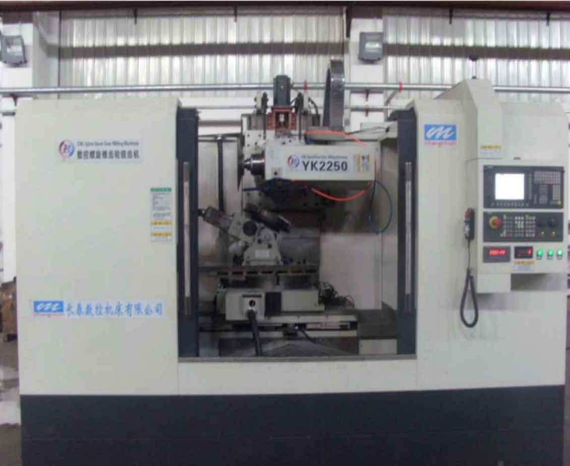
The spindle-bearing system in a spiral bevel gear milling machine typically consists of a rotating shaft supported by tapered roller bearings, driven by a torque motor, and equipped with a cutting tool assembly. During gear milling, complex spatial cutting paths generate varying loads that excite dynamic modes, potentially causing resonant vibrations. To mitigate this, we adopt a lumped mass method to discretize the continuous spindle system into equivalent mass-spring elements. This approach simplifies the analysis while capturing essential dynamic features. The system is modeled as a rotor with multiple degrees of freedom, considering translational and rotational motions. The governing equation for the undamped system is expressed as:
$$M \ddot{X} + K X = F(t)$$
where \( M \) is the mass matrix, \( K \) is the stiffness matrix, \( X \) is the displacement vector, and \( F(t) \) is the external force vector. For gear milling applications, forces include cutting loads, gravitational effects, and inertial terms from rotating components. The displacement vector typically comprises radial and axial displacements at bearing locations, which are critical for assessing vibration modes.
To derive the mass matrix, we apply the lumped mass method to the spindle assembly. The continuous shaft is divided into segments, and masses are concentrated at nodal points, particularly at bearing positions. For a shaft segment of length \( l_i \) and mass per unit length \( \mu_i \), the equivalent lumped masses at the left and right ends are calculated as:
$$m^L_j = \frac{1}{l} \sum_{k=1}^n \mu_k l_k (l – a_k), \quad m^R_j = \frac{1}{l} \sum_{k=1}^n \mu_k l_k a_k$$
where \( a_k \) is the distance from the segment centroid to the left end, and \( l \) is the total length. The total mass at a bearing node \( j \) includes the initial bearing mass and the contributions from adjacent segments. This discretization facilitates the assembly of the global mass matrix \( M \), which is diagonal for simplicity. For a system with two bearings and axial motion, the mass matrix can be represented as:
$$M = \text{diag}(m_{b1}, m_{b1}, m_{b2}, m_{b2}, m_{b1} + m_{b2})$$
where \( m_{b1} \) and \( m_{b2} \) are the equivalent masses at the left and right bearings, respectively. These masses incorporate the tool assembly, motor rotor, and other attachments, reflecting the inertial properties relevant to gear milling dynamics.
The stiffness matrix \( K \) is more complex, as it involves contributions from the spindle shaft and bearings. For the spindle rotor, we model it as a Timoshenko beam to account for shear deformation and rotational inertia, which are significant in short, thick shafts common in gear milling machines. The Timoshenko beam theory provides accurate natural frequency predictions compared to Euler-Bernoulli beams. The equation of motion for a uniform Timoshenko beam is:
$$\frac{\partial^4 y}{\partial x^4} + \frac{\mu}{EI} \frac{\partial^2 y}{\partial t^2} – \mu A \left( \frac{1}{E} + \frac{1}{Gk} \right) \frac{\partial^4 y}{\partial x^2 \partial t^2} + \frac{\mu^2}{EGAk} \frac{\partial^4 y}{\partial t^4} = 0$$
where \( E \) is Young’s modulus, \( I \) is the area moment of inertia, \( G \) is the shear modulus, \( k \) is the shear correction factor, \( \mu \) is mass per unit length, \( A \) is the cross-sectional area, and \( y \) is the transverse deflection. To derive the stiffness matrix, we consider the beam’s state variables, including displacements and slopes at the ends. Using transfer matrix methods, the relationship between forces and displacements at the left and right ends can be expressed in a stiffness form. For a beam element, the stiffness matrix \( K_s \) in local coordinates is:
$$K_s = \begin{bmatrix}
K_{s11} & K_{s12} \\
K_{s21} & K_{s22}
\end{bmatrix}$$
where submatrices involve parameters like \( \lambda_1 \) and \( \lambda_2 \), which depend on frequency and material properties. By assembling these matrices for the entire spindle, we obtain the rotor’s contribution to the global stiffness matrix.
For tapered roller bearings, which are commonly used in gear milling spindles due to their high load capacity, the stiffness is nonlinear and depends on preload and operational conditions. Under axial preload \( F_{a0} \), the bearing generates both axial and radial stiffness components. The axial stiffness \( k_a \) is defined as the ratio of axial force to axial displacement:
$$k_a = \frac{F_a}{\delta_a}$$
where \( \delta_a \) is the axial deformation. For tapered roller bearings, empirical formulas relate preload to displacement. The axial displacement can be estimated as:
$$\delta_a = \frac{6 \times 10^{-4}}{\sin \alpha} Q^{0.9} l_a^{0.8}$$
with \( Q = F_{a0} / (Z \sin \alpha) \), where \( \alpha \) is the nominal contact angle, \( Z \) is the number of rollers, and \( l_a \) is the effective roller length. This stiffness is crucial for axial vibrations during gear milling, especially when cutting forces have significant axial components.
The radial stiffness \( k_r \) is derived from load-displacement curves, considering the bearing geometry and material properties. For a tapered roller bearing under combined axial and radial loads, the radial stiffness can be expressed as:
$$k_r = \frac{\Delta F_r}{\Delta \delta_r} = \frac{1}{m \ln F_r + m + n}$$
where \( m \) and \( n \) are coefficients dependent on contact angles and material constants, and \( F_r \) is the total radial force including preload effects. Specifically, \( F_r = F_{ar} + F_{or} = F_{a0} \sin \alpha + F_{or} \), with \( F_{or} \) being the external radial load from gear milling forces. The parameters \( m \) and \( n \) are given by:
$$m = -\frac{\cos(\alpha + \beta)}{Z E’} \left( \frac{2.6}{\cos \alpha} – \frac{8.16}{\cos(\alpha + 2\beta)} \right), \quad n = -\frac{2.6 \cos(\alpha + \beta)}{Z E’ \cos \alpha}$$
where \( \beta \) is the roller half-angle, and \( E’ = E / (1 – \nu^2) \) is the effective modulus for Hertzian contact. These stiffness values are incorporated into the global stiffness matrix \( K \), which for our system is diagonal when bearing couplings are neglected:
$$K = \text{diag}(k_{b1}, k_{b1}, k_{b2}, k_{b2}, k_z)$$
where \( k_{b1} \) and \( k_{b2} \) are radial stiffnesses at the bearings, and \( k_z \) is the axial stiffness. In practice, cross-coupling terms may exist due to bearing anisotropy, but for simplicity in gear milling analysis, we assume decoupled directions.
To solve the dynamic equation, we consider free vibrations to find natural frequencies. Setting \( F(t) = 0 \), the eigenvalue problem is:
$$|K – \omega_n^2 M| = 0$$
where \( \omega_n \) are the natural frequencies. For forced vibrations during gear milling, the equation becomes \( |K – \omega^2 M| = F \), requiring numerical integration or modal superposition. The external forces in gear milling include periodic cutting forces, which can be modeled as harmonic functions. For example, radial forces might be \( F_r(t) = F_0 \cos(\omega t) \) due to tool engagement, and axial forces vary with feed motion. These excitations can lead to resonance if they coincide with natural frequencies, emphasizing the need for accurate dynamic models in gear milling machine design.
We validate the numerical model through experimental modal analysis using impact hammer testing. The spindle system is excited at key points, and accelerometers measure vibration responses. Frequency response functions are derived via Fast Fourier Transform (FFT), revealing peaks corresponding to natural frequencies. The experimental setup mimics operational conditions in gear milling, with preloads applied to bearings. Results are compared to numerical predictions from the lumped parameter model. A typical comparison for the first five natural frequencies is shown in Table 1, highlighting the model’s accuracy.
| Mode | Experimental Frequency (Hz) | Numerical Frequency (Hz) | Relative Error (%) | Numerical Frequency with Increased Preload (Hz) |
|---|---|---|---|---|
| 1 | 880.43 | 1002.53 | 13.87 | 1305.80 |
| 2 | 1805.59 | 1985.16 | 9.95 | 2013.19 |
| 3 | 2568.09 | 2769.39 | 7.84 | 2700.12 |
| 4 | 2801.92 | 2980.51 | 6.37 | 2986.57 |
| 5 | 2883.25 | 3009.12 | 4.37 | 3001.36 |
The table shows that numerical frequencies are slightly higher due to the absence of damping in the model, but errors are within acceptable limits for gear milling applications. Increasing axial preload from 3000 N to 6500 N raises natural frequencies, particularly for lower modes, which can help avoid chatter in gear milling by shifting resonances away from excitation frequencies. This underscores the importance of preload optimization in spindle design for stable gear milling processes.
To further elaborate on the dynamics, we can derive additional formulas for specific components. For instance, the equivalent mass calculation for complex geometries like tool holders can be refined using energy methods. The kinetic energy of the rotor system is:
$$E_k = \frac{1}{2} \left[ m_{b1} (\dot{x}_{b1}^2 + \dot{y}_{b1}^2) + m_{b2} (\dot{x}_{b2}^2 + \dot{y}_{b2}^2) + (m_{b1} + m_{b2}) \dot{z}^2 \right]$$
and potential energy is:
$$E_p = \frac{1}{2} \left[ k_{b1} (x_{b1}^2 + y_{b1}^2) + k_{b2} (x_{b2}^2 + y_{b2}^2) + k_z z^2 \right]$$
Applying Lagrange’s equations, we obtain the differential equations of motion. For example, the equation for radial motion at the left bearing is:
$$m_{b1} \ddot{x}_{b1} + k_{b1} x_{b1} = F_r(t)$$
where \( F_r(t) \) includes cutting forces from gear milling. These equations form the basis for time-domain simulations, which can predict transient responses during gear milling operations.
The stiffness matrix for the Timoshenko beam can be detailed further. For a beam element of length \( L \), the stiffness matrix in terms of displacements \( y \) and slopes \( \theta \) is given by:
$$K_s = \frac{EI}{L^3} \begin{bmatrix}
12 & 6L & -12 & 6L \\
6L & (4 + \phi)L^2 & -6L & (2 – \phi)L^2 \\
-12 & -6L & 12 & -6L \\
6L & (2 – \phi)L^2 & -6L & (4 + \phi)L^2
\end{bmatrix}$$
where \( \phi = 12EI/(kGA L^2) \) accounts for shear deformation. This matrix can be extended to include axial and torsional degrees of freedom, providing a comprehensive rotor model. For gear milling spindles with variable cross-sections, we segment the shaft and assemble matrices accordingly.
Regarding bearing dynamics, the tapered roller bearing stiffness can be expressed in matrix form to include coupling effects. The bearing force-displacement relationship is:
$$\begin{bmatrix} F_x \\ F_y \\ F_z \end{bmatrix} = \begin{bmatrix} k_{xx} & k_{xy} & k_{xz} \\ k_{yx} & k_{yy} & k_{yz} \\ k_{zx} & k_{zy} & k_{zz} \end{bmatrix} \begin{bmatrix} \delta_x \\ \delta_y \\ \delta_z \end{bmatrix}$$
where off-diagonal terms represent cross-coupling due to bearing geometry. For simplicity, we often assume \( k_{xx} = k_{yy} = k_r \) and \( k_{zz} = k_a \), with others zero. However, in precision gear milling, these couplings may influence vibration modes and should be considered in advanced models.
To enhance the model for gear milling applications, we incorporate cutting force models. The forces during spiral bevel gear milling depend on tool geometry, material properties, and cutting parameters. A typical force model includes tangential, radial, and axial components:
$$F_t = K_t a_p f, \quad F_r = K_r F_t, \quad F_a = K_a F_t$$
where \( K_t, K_r, K_a \) are specific cutting coefficients, \( a_p \) is depth of cut, and \( f \) is feed rate. These forces act as excitations in the dynamic equation, potentially leading to chatter if the system is unstable. The stability lobe diagram can be derived by solving the delayed differential equations that account for regenerative effects in gear milling. The critical depth of cut for chatter is:
$$a_{p,\text{lim}} = -\frac{1}{2K_t \text{Re}(G(\omega))}$$
where \( G(\omega) \) is the frequency response function of the spindle system. This highlights the interplay between dynamics and machining parameters in gear milling.
We also explore damping effects, though our primary model is undamped. In reality, material damping, bearing damping, and interface damping dissipate energy. A proportional damping model can be added as \( C = \alpha M + \beta K \), where \( \alpha \) and \( \beta \) are coefficients. The damped equation becomes:
$$M \ddot{X} + C \dot{X} + K X = F(t)$$
This allows for more accurate predictions of vibration amplitudes during gear milling, especially near resonances.
For numerical solution, we use subspace iteration or finite element methods to extract modes. The natural frequencies and mode shapes inform design modifications, such as adjusting bearing positions or preloads. In gear milling machines, optimizing the spindle-bearing system can reduce chatter risk and improve surface quality. Table 2 summarizes key parameters used in our analysis for a typical gear milling spindle.
| Parameter | Symbol | Value | Unit |
|---|---|---|---|
| Shaft length | L | 0.8 | m |
| Shaft diameter | D | 0.1 | m |
| Young’s modulus | E | 210 | GPa |
| Shear modulus | G | 80 | GPa |
| Bearing contact angle | α | 15 | ° |
| Number of rollers | Z | 20 | – |
| Axial preload | F_{a0} | 3000-6500 | N |
| Tool mass | m_t | 5 | kg |
| Motor mass | m_m | 10 | kg |
| Cutting force coefficient | K_t | 2000 | N/mm² |
These parameters are used in simulations to predict dynamic behavior. For instance, the first bending mode of the spindle often occurs around 1000 Hz, which is within the excitation range of gear milling cutters operating at high speeds. By adjusting preload, we can shift this frequency higher, as shown in Table 1, reducing the likelihood of resonance during gear milling.
In conclusion, the dynamic analysis of spindle-bearing systems in spiral bevel gear milling machines is essential for ensuring machining stability and precision. Our lumped parameter model, incorporating Timoshenko beam theory and nonlinear bearing stiffness, provides a reliable tool for predicting natural frequencies and response to gear milling forces. Experimental validation confirms the model’s accuracy, with errors within practical limits. Key findings include the significant effect of axial preload on system stiffness and the importance of damping in real-world applications. Future work could involve integrating thermal effects from gear milling into the model, as temperature changes alter material properties and bearing clearances. Additionally, advanced control strategies can be developed using this model to actively suppress vibrations during gear milling, further enhancing productivity and quality in gear manufacturing.
Overall, this analysis underscores the critical role of dynamics in gear milling processes and offers a framework for optimizing spindle designs. By repeatedly considering gear milling conditions throughout the model development, we ensure relevance to real-world machining challenges. The use of formulas and tables facilitates clear communication of complex relationships, aiding engineers in designing robust systems for high-performance gear milling applications.