
In my research, I focus on the dynamic behavior and multi-objective optimization of modified helical gear transmission systems. Helical gears are widely used in mechanical transmissions because they offer better meshing performance, larger contact ratios, and more compact structures than spur gears. However, the presence of a helix angle makes the calculation of time-varying meshing stiffness (TVMS) much more complex. Most existing analytical methods were developed for spur gears, and they often ignore the actual difference between the base circle and the root circle, as well as the variation in meshing timing. Therefore, I proposed an improved analytical method to calculate the TVMS of modified helical gears, and I built a dynamic model to study their dynamic characteristics. Based on the results, I further established a multi-objective optimization model using the NSGA-II algorithm to reduce dynamic meshing force and dynamic transmission error. The overall goal is to improve the reliability, reduce vibration and noise, and extend the service life of helical gear transmission systems.
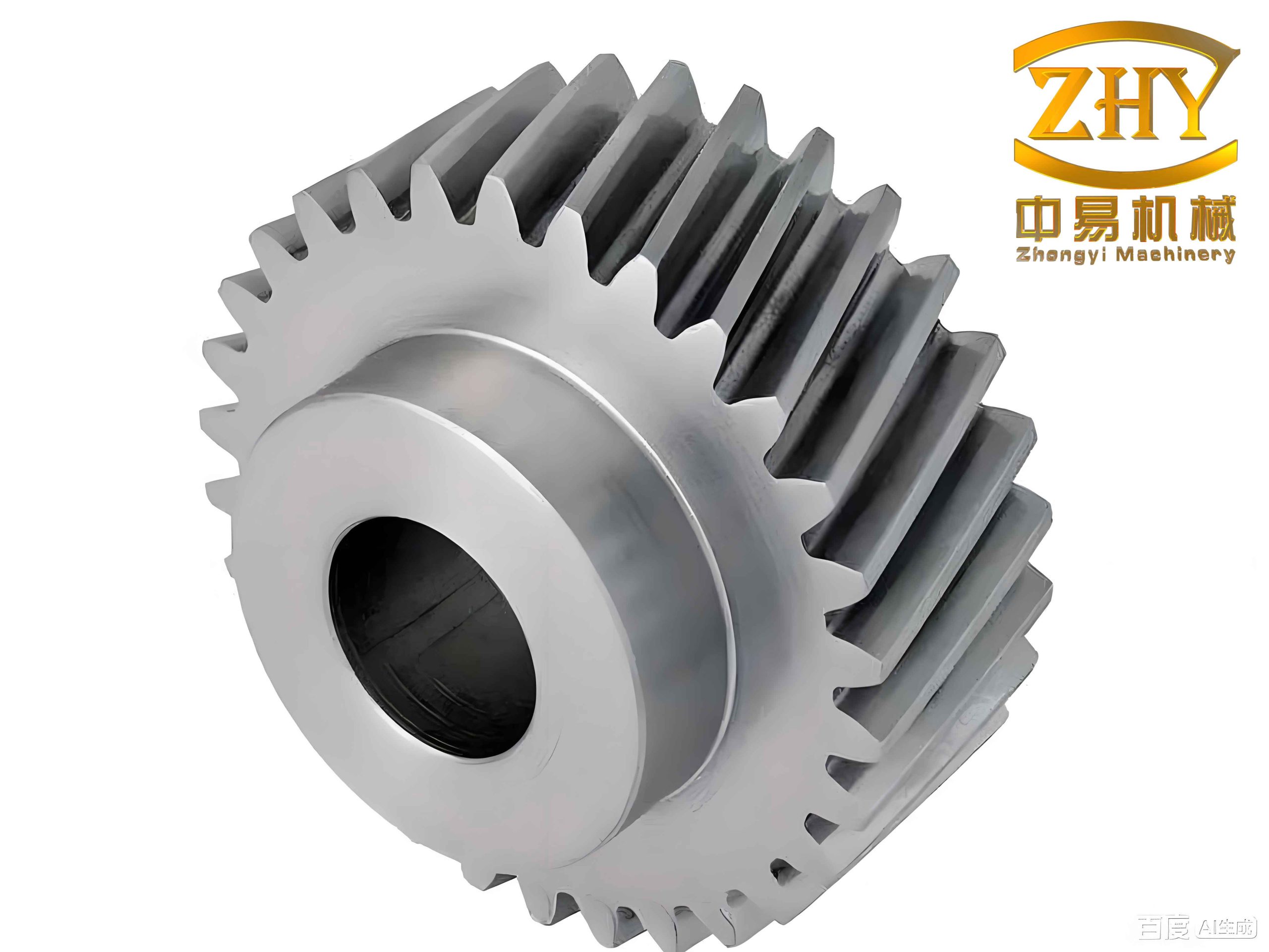
1. Time-Varying Meshing Stiffness Calculation for Helical Gears
The time-varying meshing stiffness of helical gears is a major internal excitation source in gear transmission systems. It directly affects the dynamic meshing force, dynamic transmission error, and vibration acceleration. To calculate the TVMS accurately, I adopted the slice theory and the integration concept. In this method, a helical gear is cut into many thin slices along the tooth width direction. Each slice is approximately treated as a spur gear. Then the meshing stiffness of each slice is calculated, and the single-tooth TVMS is obtained by integration. The contact line of helical gears is not parallel to the axis because of the helix angle. The length of the contact line changes continuously during meshing. This variation must be considered to obtain the correct TVMS.
The contact line length of helical gears can be expressed as a piecewise function. Let \(l\) be the contact line length, \(L\) the tooth width, \(\beta_b\) the base helix angle, and \(\mu\) the distance from the meshing start point. The function is given by:
$$ l = \begin{cases} \mu \cot \beta_b, & 0 \leq \mu \leq L \tan \beta_b \\ L, & L \tan \beta_b < \mu \leq L_1 \\ (L_1 + L_2 – \mu)\cot \beta_b, & L_1 < \mu \leq L_1 + L_2 \end{cases} $$
where the parameters are defined as:
$$ \mu = \frac{2\pi \epsilon_\alpha}{Z} \theta_1, \quad L_2 = L \tan \beta_b, \quad p_{bt} = \pi m_n \cos \alpha_t / \cos \beta_b, \quad L_1 = \frac{p_{bt} \epsilon_\alpha}{2} – L_2 $$
Here, \(Z\) is the number of teeth, \(\theta_1\) is the rotation angle of the driving gear, \(\epsilon_\alpha\) is the transverse contact ratio, \(m_n\) is the normal module, \(\alpha_t\) is the transverse pressure angle, and \(\beta_b\) is the base helix angle. The transverse pressure angle and base helix angle satisfy:
$$ \tan \alpha_t = \tan \alpha_n / \cos \beta, \quad \tan \beta_b = \tan \beta \cos \alpha_t $$
For the \(i\)-th slice, the meshing angle of the driving gear and the driven gear can be calculated based on the rotation angle and the transmission ratio. This provides the geometric basis for calculating the stiffness of each slice. I considered two cases: when the base circle radius is larger than the root circle radius, and when the base circle radius is smaller than the root circle radius. The latter case requires extending the cantilever beam, which increases the tooth deformation and reduces the stiffness.
The total deformation energy of a gear tooth includes Hertz contact energy, bending energy, shear energy, and axial compressive energy. The corresponding stiffness components are Hertz contact stiffness \(k_h\), bending stiffness \(k_b\), shear stiffness \(k_s\), axial compressive stiffness \(k_a\), and fillet foundation stiffness \(k_f\). For a single tooth, the TVMS is obtained by combining these stiffness components in series and parallel. The formula for the single-tooth TVMS is:
$$ k = \frac{1}{\frac{1}{k_h} + \frac{1}{k_{b1}} + \frac{1}{k_{s1}} + \frac{1}{k_{a1}} + \frac{1}{k_{f1}} + \frac{1}{k_{b2}} + \frac{1}{k_{s2}} + \frac{1}{k_{a2}} + \frac{1}{k_{f2}}} $$
where the subscripts 1 and 2 refer to the driving gear and the driven gear, respectively. Each stiffness component is calculated by summing the contributions of all slices. For example, the bending stiffness \(k_b\) is given by:
$$ k_b = \sum_{i=1}^{N} \left[ \int_{\alpha_1}^{\alpha_2} \frac{3(1+\cos\alpha_1[(\alpha_2-\alpha)\sin\alpha – \cos\alpha])^2 (\alpha_2-\alpha)\cos\alpha}{2E h(y)^3} dy \right]^{-1} $$
Similar expressions are used for shear stiffness and axial compressive stiffness. The Hertz contact stiffness is:
$$ k_h = \frac{\pi E B}{4(1-\nu^2)} $$
where \(E\) is the elastic modulus, \(B\) is the face width, and \(\nu\) is the Poisson ratio. The fillet foundation stiffness is calculated using a semi-empirical formula:
$$ \frac{1}{k_f} = \frac{\cos^2 \alpha_1}{E B} \left[ L_f \left( \frac{u_f}{S_f} \right)^2 + M_f \left( \frac{u_f}{S_f} \right) + P_f (1 + Q_f \tan^2 \alpha_1) \right] $$
After obtaining the single-tooth TVMS, I considered the meshing sequence of helical gears. The total contact ratio of helical gears is \(\epsilon = \epsilon_\alpha + \epsilon_\beta\), where \(\epsilon_\beta = B \sin \beta / (\pi m_n)\) is the axial contact ratio. For a total contact ratio between 2 and 3, the gear pair experiences alternating double-tooth and triple-tooth meshing regions. The comprehensive TVMS is obtained by summing the stiffness of all simultaneously meshing teeth. A typical meshing cycle can be divided into five stages. The comprehensive TVMS is expressed as:
$$ k_m = \begin{cases} \sum_{i=1}^{2} \frac{1}{k_i}, & \text{double-tooth meshing} \\ \sum_{i=1}^{3} \frac{1}{k_i}, & \text{triple-tooth meshing} \end{cases} $$
This method provides a complete calculation framework for the TVMS of helical gears, and it will be used as the basis for the modified helical gear analysis.
2. Analytical Model for Modified Helical Gears
Modification, or shift, is an effective way to improve the load capacity and fatigue life of helical gears. The modification coefficient changes the tooth profile and the center distance. In my research, I established an analytical model for the TVMS of modified helical gears. The modification changes the addendum, dedendum, center distance, and transverse meshing angle. The addendum and dedendum are:
$$ h_{ai} = (h_a^* + x_{ni} – \Delta y_n) m_n, \quad h_{fi} = (h_a^* + c^* – x_{ni}) m_n $$
where \(h_a^*\) is the addendum coefficient, \(c^*\) is the clearance coefficient, \(x_{ni}\) is the modification coefficient, and \(\Delta y_n\) is the addendum reduction coefficient. The center distance and transverse meshing angle for a modified gear pair are:
$$ a’ = \frac{(Z_1 + Z_2) m_t \cos \alpha_t}{2 \cos \alpha_t’}, \quad \text{inv} \alpha_t’ = \text{inv} \alpha_t + \frac{2 \tan \alpha_n (x_1 + x_2)}{Z_1 + Z_2} $$
where \(m_t\) is the transverse module, \(\alpha_t\) is the transverse pressure angle, and \(\alpha_t’\) is the transverse meshing angle after modification. The initial meshing pressure angle for the driving and driven gears can be calculated from the base circle radius, addendum circle radius, and center distance.
I used the following basic parameters for a helical gear pair from a subway gearbox application:
| Parameter | Value |
|---|---|
| Normal module \(m_n\) | 5.5 mm |
| Number of teeth \(Z_1 / Z_2\) | 17 / 107 |
| Normal pressure angle \(\alpha_n\) | 20° |
| Helix angle \(\beta\) | 17° |
| Elastic modulus \(E\) | 2.06 × 10¹¹ Pa |
| Poisson ratio \(\nu\) | 0.3 |
| Addendum coefficient \(h_a^*\) | 1 |
| Clearance coefficient \(c^*\) | 0.25 |
| Face width \(L\) | 70 mm |
For single-tooth modification, I selected modification coefficients of -0.4, -0.2, 0, 0.2, and 0.4. The results show that when the gear has positive modification, the TVMS amplitude decreases as the modification coefficient increases. The reason is that the transverse contact ratio decreases, which shortens the single-tooth meshing period and reduces the effective contact length. For negative modification, the TVMS amplitude increases as the negative modification coefficient increases. The contact ratio increases, and the meshing period becomes longer. The bending stiffness, shear stiffness, and axial compressive stiffness all show a trend of first increasing and then decreasing. Positive modification makes the tooth root wider, so the stiffness components are larger than those of the standard gear. Negative modification makes the tooth root narrower, so the stiffness components are smaller.
For compound modification, I considered equal compound shift and unequal compound shift. In equal compound shift, the driving gear uses positive modification and the driven gear uses negative modification. I analyzed cases with driving gear coefficients of 0, 0.1, 0.2, 0.3 and driven gear coefficients of 0, -0.1, -0.2, -0.3. The TVMS increases as the driving gear modification coefficient increases and the driven gear modification coefficient decreases. The triple-tooth meshing region becomes shorter, and the double-tooth meshing region becomes longer. The mean value and standard deviation both increase. The fluctuation factor also increases.
For unequal compound shift, I studied positive transmission and negative transmission. In positive transmission, the driving gear coefficient is fixed at 0.3, and the driven gear coefficient varies from -0.2 to 0.2. The TVMS decreases as the driven gear modification coefficient increases. The mean value, standard deviation, and fluctuation factor all decrease. In negative transmission, the driving gear coefficient is fixed at -0.3, and the driven gear coefficient varies from -0.2 to 0.2. The TVMS also decreases as the driven gear modification coefficient increases. The mean value and standard deviation decrease, and the fluctuation factor decreases.
To quantify the TVMS variation, I used the mean value, standard deviation, and comprehensive stiffness fluctuation factor. These are defined as:
$$ K_a = \text{mean}(K_m), \quad K_{STD} = \sqrt{\frac{1}{N}\sum_{i=1}^{N}(K_{mi} – K_a)^2}, \quad \Delta K = \frac{K_{max} – K_{min}}{K_a} $$
These indicators provide a comprehensive evaluation of the stability and reliability of the gear transmission.
To validate the analytical model, I used the finite element method. I built a 3D model of the modified helical gear pair and imported it into ABAQUS. The contact was defined as frictional contact with a friction coefficient of 0.2. The driven gear was fixed, and the driving gear was allowed to rotate about its axis. A torque of 1000 N·m was applied. The comparison between my analytical method and the finite element method showed very good agreement, with a maximum error of about 1%. This confirms that my analytical model is accurate and effective for calculating the TVMS of modified helical gears.
3. Dynamic Modeling of the Modified Helical Gear Transmission System
To study the dynamic characteristics of the modified helical gear transmission system, I established an eight-degree-of-freedom dynamic model. The model considers three translational directions and one rotational direction for both the driving gear and the driven gear. The generalized displacement vector is:
$$ q = \{x_p, y_p, z_p, \theta_p, x_g, y_g, z_g, \theta_g\}^T $$
where the subscripts \(p\) and \(g\) denote the driving gear and the driven gear, respectively. The dynamic model is based on Lagrange’s equation. The kinetic energy, potential energy, and dissipation function are used to derive the equations of motion. The dynamic meshing force is:
$$ F_m = k_m \cdot DTE + c_m \cdot \dot{DTE} $$
where \(k_m\) is the comprehensive TVMS, and \(c_m\) is the meshing damping coefficient. The damping coefficient is calculated as \(c_m = 2\xi \sqrt{\bar{k}_m m}\), where \(\xi\) is the damping ratio, \(\bar{k}_m\) is the average meshing stiffness, and \(m\) is the equivalent mass. The dynamic transmission error (DTE) is defined as:
$$ DTE = (x_p – x_g)\cos\beta_b + (y_p – y_g)\sin\beta_b + (\theta_p R_p – \theta_g R_g)\cos\beta_b – e(t) $$
where \(R_p\) and \(R_g\) are the base circle radii, and \(e(t)\) is the static transmission error. The equations of motion for the driving gear are:
$$ m_p \ddot{x}_p + c_{px} \dot{x}_p + k_{px} x_p = -F_m \cos\beta_b \cos\alpha_t – F_f \sin\alpha_t $$
$$ m_p \ddot{y}_p + c_{py} \dot{y}_p + k_{py} y_p = -F_m \cos\beta_b \sin\alpha_t – F_f \cos\alpha_t $$
$$ m_p \ddot{z}_p + c_{pz} \dot{z}_p + k_{pz} z_p = -F_m \sin\beta_b $$
$$ I_p \ddot{\theta}_p = F_m R_p – T_p $$
Similar equations are written for the driven gear. The friction force is calculated based on the slice model. The total friction force is the sum of the friction forces on all slices. The dynamic model is solved numerically to obtain the time-domain and frequency-domain responses.
To verify the dynamic model, I built an experimental platform. The helical gear pair used in the experiment had the same parameters as those in the analytical model. The driving gear modification coefficient was 0.2803, and the driven gear modification coefficient was -0.2803. A vibration acceleration sensor was installed on the driven gear end cover. The experiment was conducted under uniform speed conditions. The comparison between the simulation and experimental results showed that the amplitudes were very close, with only small differences due to environmental noise. This confirms that my dynamic model is accurate and effective.
4. Dynamic Characteristics Analysis
Using the verified dynamic model, I analyzed the dynamic meshing force, dynamic transmission error, and axial vibration acceleration under different modification conditions and rotational speeds. I used two time-domain indicators: root mean square (RMS) and kurtosis value (KV). The RMS is defined as:
$$ X_{rms} = \sqrt{\frac{1}{N}\sum_{i=1}^{N} x_i^2} $$
The kurtosis is:
$$ X_{kv} = \frac{1}{N}\sum_{i=1}^{N} \left( \frac{x_i – \bar{x}}{\sigma} \right)^4 $$
To compare the results clearly, I normalized the indicators as:
$$ Y_S = \frac{Y_i – Y_0}{Y_0} \times 100\% $$
where \(Y_S\) is the modified indicator, \(Y_i\) is the indicator for the modified gear, and \(Y_0\) is the indicator for the standard gear.
For the dynamic meshing force, I found that when the gear pair has positive transmission, the dynamic meshing force decreases compared with the standard gear. The time-domain amplitude and fluctuation are smaller. In the frequency domain, the meshing frequency and its harmonics decrease, and the sidebands are reduced. For negative transmission, the opposite trend is observed. The dynamic meshing force increases, and the sidebands become more numerous. When the rotational speed increases from 1000 rpm to 5000 rpm, the meshing frequency amplitude increases significantly for all cases. The positive transmission gear always has a smaller meshing frequency amplitude than the standard gear, while the negative transmission gear always has a larger one. The positive transmission gear has a more significant effect on the dynamic meshing force at higher speeds.
| Modification type | Dynamic meshing force | Dynamic transmission error | Axial vibration acceleration |
|---|---|---|---|
| Positive transmission | Decreases | Increases | Decreases |
| Standard gear | Reference | Reference | Reference |
| Negative transmission | Increases | Decreases | Increases |
For the dynamic transmission error, I observed that positive transmission increases the DTE, while negative transmission decreases it. The DTE reflects the transmission accuracy and stability. A smaller DTE means better precision. In the frequency domain, positive transmission increases the meshing frequency and its harmonics, and the envelope period becomes longer, leading to more sidebands. Negative transmission reduces the meshing frequency and shortens the envelope period, leading to fewer sidebands. When the rotational speed increases from 1000 rpm to 5000 rpm, the DTE meshing frequency amplitude increases significantly. The negative transmission gear has a more significant effect on the DTE at higher speeds.
For the axial vibration acceleration, I found that positive transmission decreases the axial vibration acceleration, while negative transmission increases it. The axial force is an important factor affecting the vibration characteristics of helical gears. The driving gear is more sensitive to axial force changes because it directly bears the load. Therefore, I focused on the axial vibration acceleration of the driving gear. The time-domain and frequency-domain results show that positive transmission reduces the vibration amplitude, while negative transmission increases it. When the rotational speed increases from 1000 rpm to 5000 rpm, the axial vibration acceleration meshing frequency amplitude increases significantly. The positive transmission gear has a more significant effect on the axial vibration acceleration at higher speeds.
In summary, the modification coefficient has a strong influence on the dynamic characteristics of helical gear transmission systems. Positive transmission reduces the dynamic meshing force and axial vibration acceleration but increases the dynamic transmission error. Negative transmission reduces the dynamic transmission error but increases the dynamic meshing force and axial vibration acceleration. These findings provide a theoretical basis for optimizing the modification coefficients.
5. Multi-Objective Optimization Using NSGA-II
To improve the dynamic performance of the modified helical gear transmission system, I established a multi-objective optimization model. The design variables are the modification coefficients of the driving gear and the driven gear. The objective functions are to minimize the dynamic meshing force and minimize the dynamic transmission error. The constraints are based on the recommended range of modification coefficients:
$$ 0 < x_p \leq 0.4, \quad -0.4 \leq x_g < 0 $$
The optimization model is:
$$ \text{Min. } f_1(X) = RMS(F_m), \quad \text{Min. } f_2(X) = RMS(DTE) $$
$$ \text{S.t. } 0 < x_p \leq 0.4, \quad -0.4 \leq x_g < 0, \quad X = [x_p, x_g]^T $$
I used the NSGA-II algorithm to solve this multi-objective optimization problem. The algorithm parameters were set as follows: population size 50, maximum generations 20, crossover probability 0.9, and mutation probability 0.1. The Pareto optimal solution set was obtained after 20 generations. Each point in the Pareto front represents a trade-off between the two objectives. I selected a compromise solution that balances low dynamic force and low transmission error.
For the low rotational speed condition (1000 rpm), the selected optimal modification coefficients were \(x_p = 0.0855\) and \(x_g = -0.3867\). Under these coefficients, the RMS of the dynamic meshing force decreased by 2.5402%, and the RMS of the dynamic transmission error decreased by 6.9525%. The axial vibration acceleration also decreased. The time-domain and frequency-domain responses confirmed the improvement. For comparison, other Pareto optimal points were also analyzed. The results are summarized in the table below.
| Condition | Parameter | Before optimization | After optimization (A) | After optimization (B) | After optimization (C) |
|---|---|---|---|---|---|
| Low speed (1000 rpm) | Driving gear \(x_p\) | 0.2803 | 0.1188 | 0.0855 | 0.0697 |
| Driven gear \(x_g\) | -0.2803 | -0.3085 | -0.3867 | -0.3923 | |
| RMS of \(F_m\) (N) | 7.7572 × 10⁴ | 7.4509 × 10⁴ | 7.5602 × 10⁴ | 7.6781 × 10⁴ | |
| RMS of DTE (mm) | 1.0486 × 10⁻² | 1.0033 × 10⁻² | 0.9757 × 10⁻² | 0.9675 × 10⁻² | |
| High speed (5000 rpm) | Driving gear \(x_p\) | 0.2803 | 0.0673 | 0.1129 | 0.1256 |
| Driven gear \(x_g\) | -0.2803 | -0.3057 | -0.3616 | -0.3929 | |
| RMS of \(F_m\) (N) | 7.7946 × 10⁴ | 7.3969 × 10⁴ | 7.4106 × 10⁴ | 7.4326 × 10⁴ | |
| RMS of DTE (mm) | 1.0536 × 10⁻² | 1.0034 × 10⁻² | 0.9715 × 10⁻² | 0.9598 × 10⁻² |
For the high rotational speed condition (5000 rpm), the selected optimal modification coefficients were \(x_p = 0.1129\) and \(x_g = -0.3616\). Under these coefficients, the RMS of the dynamic meshing force decreased by 4.9271%, and the RMS of the dynamic transmission error decreased by 7.8796%. The axial vibration acceleration also decreased. The optimization results at high speed show that the system achieves low dynamic force and low transmission error simultaneously. The comparison with the pre-optimization results confirms that the dynamic performance of the helical gear transmission system is effectively improved.
The optimization process demonstrates that the NSGA-II algorithm is effective for solving the multi-objective optimization problem of modified helical gears. The Pareto front provides a set of optimal solutions, and the decision maker can select the most suitable one according to the specific requirements. The results also show that the modification coefficients have a significant impact on the dynamic characteristics of helical gears. By properly selecting the modification coefficients, the dynamic meshing force and dynamic transmission error can be reduced, and the axial vibration acceleration can also be decreased.
6. Conclusions and Future Work
In my research, I proposed an analytical method for calculating the time-varying meshing stiffness of modified helical gears. The method is based on slice theory and integration, and it considers the actual difference between the base circle and the root circle, as well as the variation in meshing timing. I established an analytical model and validated it using the finite element method. The results show that the modification coefficient has a strong influence on the TVMS. For single-tooth modification, the TVMS amplitude and contact ratio are negatively correlated with the modification coefficient. For equal compound shift, the TVMS amplitude is positively correlated with the driving gear modification coefficient and negatively correlated with the driven gear modification coefficient. For unequal compound shift, the TVMS amplitude is negatively correlated with the modification coefficient.
I also established an eight-degree-of-freedom dynamic model for the modified helical gear transmission system. The model was validated by experiments. The dynamic characteristics were analyzed under different modification conditions and rotational speeds. The results show that positive transmission reduces the dynamic meshing force and axial vibration acceleration but increases the dynamic transmission error. Negative transmission reduces the dynamic transmission error but increases the dynamic meshing force and axial vibration acceleration. As the rotational speed increases, the meshing frequency and amplitude of the dynamic meshing force, dynamic transmission error, and axial vibration acceleration all increase significantly. The positive transmission gear has a more significant effect on the dynamic meshing force and axial vibration acceleration at higher speeds, while the negative transmission gear has a more significant effect on the dynamic transmission error.
Finally, I established a multi-objective optimization model to minimize the dynamic meshing force and dynamic transmission error. The NSGA-II algorithm was used to solve the model. The optimal modification coefficients were obtained for both low and high rotational speed conditions. The results show that the optimized system has lower dynamic meshing force, lower dynamic transmission error, and lower axial vibration acceleration. This provides an effective method for the optimization of modified helical gear transmission systems.
For future work, I plan to extend the optimization to include more parameters, such as the helix angle, module, and pressure angle. I also plan to consider the influence of the gearbox housing on the dynamic characteristics. This will make the analysis more comprehensive and closer to real engineering applications. The dynamic behavior and optimization of helical gears will continue to be an important research direction in mechanical engineering.