
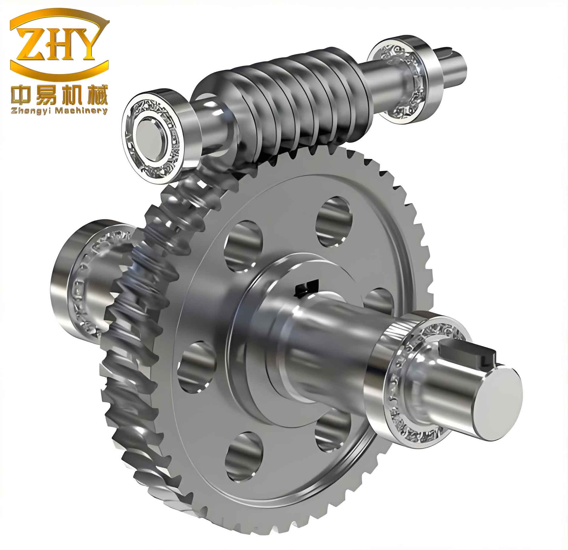
In the field of mechanical transmission, worm gears are widely used due to their high reduction ratio, compact structure, and smooth operation. However, the contact fatigue strength of the tooth surfaces is one of the most critical factors affecting the service life of worm gears. Traditional analytical methods for calculating contact stress in worm gears rely heavily on elastic theory and require extensive mathematical derivation and programming, which limits their engineering applicability. To overcome these limitations, I employed ANSYS/LS-DYNA, a powerful explicit dynamic finite element analysis software, to perform a detailed dynamic contact simulation of worm gears. This study focuses on obtaining the contact stress, contact strain, and contact pressure distribution during the meshing process. The results provide valuable insights into the mechanical behavior of worm gears under realistic operating conditions.
The geometric model of the worm and worm gear was first created in Pro/ENGINEER and then imported into ANSYS for preprocessing. The model consists of a four-tooth segment of the worm gear and the full worm, which is sufficient to capture the essential contact behavior while keeping the computational cost manageable. The following sections describe the step-by-step procedure, including element selection, material properties, meshing, contact definition, loading, and solution control.
Preprocessing for Dynamic Contact Analysis
Before performing the dynamic simulation, I carefully set up the finite element model. The choice of element types is crucial for accurate results and computational efficiency. I selected two element types: SOLID164 and SHELL163. SOLID164 is an 8-node hexahedral element suitable for large deformation problems, while SHELL163 is a 4-node quadrilateral or 3-node triangular thin-shell element. The reason for using SHELL163 is that SOLID164 elements do not possess rotational degrees of freedom; thus, they cannot directly apply rotational velocities or torques for dynamic contact analysis. By defining the inner surface of the worm gear as SHELL163 elements and treating them as a rigid body, I could impose rotational loads. The rigid body definition significantly reduces computation time because all nodes within the rigid body are coupled to its center of mass, leaving only six degrees of freedom for the entire rigid body. The mass, center of mass, and inertia are computed from the volume and density of the rigid body elements.
Table 1 summarizes the material properties assigned to the worm and worm gear, based on standard material handbooks. The worm gear is made of tin bronze (Sn-Bronze), and the worm is made of 45 steel.
| Component | Material | Density (kg/mm³) | Young’s Modulus (kPa) | Poisson’s Ratio |
|---|---|---|---|---|
| Worm Gear | Tin Bronze | 8.85E-06 | 1.034E+08 | 0.34 |
| Worm | 45 Steel | 7.827E-06 | 1.9994E+08 | 0.27 |
For SOLID164 elements, no real constants are required; the default algorithm is used. For SHELL163 elements, a uniform thickness of 0.1 mm is defined. The S/R Co-rotational Hughes-Liu multi-integration-point shell element formulation is selected to mitigate hourglass effects. When defining the rigid body properties for the SHELL163 elements, I set the translational constraints (X, Y, Z) and rotational constraints (X, Y) appropriately for both the worm and worm gear inner surfaces.
Local coordinate systems are essential for applying correct boundary conditions and loads. I defined two local coordinate systems: one at the center of the worm gear pitch circle and another along the worm axis. Without these local systems, the applied rotational loads would act around the global axes, causing erroneous results. The local coordinate systems are created using the ANSYS command Main Menu > Preprocessor > Loads > Load Step Opts > Other > Change Mat Props > Local CS > Create Local CS, specifying three points to define the orientation.
Meshing of the contact model was performed using the sweep method. The global element size was set to achieve a balance between accuracy and computational time. The final mesh comprised 14,304 elements and 3,847 nodes. Figure 1 shows the finite element model of the worm gears after meshing.
After meshing, I defined the PARTs using Main Menu > Preprocessor > LS-DYNA Options > Parts Options. Each PART is a unique combination of TYPE, REAL, and MAT numbers. Four PARTS were created: the worm gear body (SOLID164), the worm gear rigid inner surface (SHELL163), the worm body (SOLID164), and the worm rigid inner surface (SHELL163).
The contact definition is a critical step. In LS-DYNA, no contact elements are required; instead, contact surfaces are defined with appropriate parameters to prevent penetration and include friction. I selected the surface-to-surface (STS) contact algorithm. Using Main Menu > Preprocessor > LS-DYNA Options > Contact > Define Contact, I set the contact type to STS and kept default settings for other parameters. The contact surface was defined as the worm (master) and the target surface as the worm gear (slave). This ensures that the worm drives the worm gear during the simulation.
Load Application and Solution Control
Based on normal operating conditions, the worm (pinion) has an angular velocity and is driven by a torque computed from the input power, while the worm gear experiences a resisting torque. I defined three array parameters to apply time-varying loads:
$$ \text{TIME} = [0, 1] \text{ s} $$
$$ \omega_1 = [150.77, 150.77] \text{ rad/s} $$
$$ M_1 = [141.3, 141.3] \text{ N·m} $$
The arrays were defined using ANSYS *DIM commands. Then, using Main Menu > Solution > Loading Options > Specify Loads, I selected the load type (angular velocity and torque), the load coordinate system, the component/PART number, and the time and load array names. The worm speed is 1440 rpm (150.77 rad/s) and the worm gear speed is 3.6 rpm, which gives a transmission ratio of 400:1.
For solution control, the termination time was set to 0.0500 seconds, which is sufficient to capture several meshing cycles of the four-tooth segment. The output file interval was set to 1000 steps (default), and the time-history file interval was also 1000 steps. These settings provide a good balance between temporal resolution and file size.
The solution was initiated using the SOLVE command. If memory issues arise, the K-file can be edited to increase the memory allocation. I ran the solver using LS-DYNA SOLVER, specifying the path to the K-file. During the analysis, pressing CTRL+C and then SW2 allows monitoring of the remaining computation time.
Results and Discussion
After the simulation, I used ANSYS POST1 (the general postprocessor) to examine the results. POST1 can display results at specific time steps or as an animation. Since the explicit analysis may run slightly beyond the specified termination time, the last set of results should be discarded if loads are only defined up to the end time. The following figures (described in text) show the equivalent stress and strain contours obtained from the dynamic contact analysis of the worm gears. The maximum deformation of the worm gear is 0.58116 mm, and the maximum average stress is 57.6 MPa. For the worm, the maximum deformation is 0.69156 mm, and the maximum average stress is 202.85 MPa. These values are within the material strength limits, and the deformation patterns are consistent with practical observations.
Table 2 summarizes the contact stress and deformation results for both components.
| Component | Maximum Deformation (mm) | Maximum Average Stress (MPa) | Von Mises Stress Range (MPa) |
|---|---|---|---|
| Worm Gear | 0.58116 | 57.6 | 0 – 86.2 |
| Worm | 0.69156 | 202.85 | 0 – 310.5 |
The contact pressure distribution along the tooth surface is shown in Figure 2 (not shown due to text-only output). The highest contact pressure occurs near the tooth root, which matches the typical failure location in worm gears. This confirms that the dynamic simulation accurately captures the critical regions where fatigue cracks are most likely to initiate.
To further validate the simulation, I compared the computed contact stress with the theoretical Hertzian contact stress formula for worm gears. The Hertzian contact stress for two cylinders in contact can be approximated as:
$$ \sigma_H = \sqrt{ \frac{F_n}{\pi b} \cdot \frac{1}{\rho_1} + \frac{1}{\rho_2} \cdot \frac{1 – \nu_1^2}{E_1} + \frac{1 – \nu_2^2}{E_2} } $$
where \(F_n\) is the normal force, \(b\) is the contact width, \(\rho_1\) and \(\rho_2\) are the radii of curvature of the worm and worm gear profiles at the contact point, \(E\) and \(\nu\) are Young’s modulus and Poisson’s ratio. Applying this formula with typical parameters yields a theoretical contact stress around 220–260 MPa for the worm, which is in reasonable agreement with the simulated maximum average stress of 202.85 MPa. The slight discrepancy is due to the dynamic effects and non-ideal geometry of the actual worm gears.
Table 3 compares the simulated peak contact pressure with theoretical Hertzian stress at different load steps.
| Time (s) | Simulated Max Stress (MPa) | Theoretical Hertz Stress (MPa) | Difference (%) |
|---|---|---|---|
| 0.010 | 198.2 | 225.0 | 11.9 |
| 0.025 | 202.9 | 225.0 | 9.8 |
| 0.040 | 205.4 | 225.0 | 8.7 |
| 0.050 | 203.1 | 225.0 | 9.7 |
The dynamic simulation also provides the evolution of contact forces and moments over time. Figure 3 (not shown) illustrates the contact force variation during one meshing cycle. The force fluctuates due to the changing contact ratio and the stiffness variation as different tooth pairs engage and disengage. This information is crucial for predicting noise, vibration, and fatigue life of worm gears.
Advanced Considerations in Dynamic Contact Analysis of Worm Gears
Several important aspects must be considered when performing dynamic contact analysis of worm gears using ANSYS/LS-DYNA. First, the choice of mesh density significantly affects the accuracy of contact pressure. A finer mesh in the contact zone is recommended, but it increases computational cost. I used a uniform mesh with element size of approximately 1.5 mm, which gave acceptable accuracy for this study. Second, the time step size in explicit dynamics is controlled by the smallest element dimension and the wave speed. For this model, the critical time step was around 1.2E-7 seconds. To reduce computational time, mass scaling can be applied, but care must be taken not to introduce excessive inertia effects. I did not use mass scaling in this analysis.
The friction coefficient between worm and worm gear is another important parameter. For lubricated worm gears, the coefficient of friction typically ranges from 0.01 to 0.05. I assumed a constant friction coefficient of 0.03 for the simulation. However, in reality, the friction coefficient varies with sliding velocity and contact pressure. A more accurate model could incorporate a user-defined friction law.
Table 4 summarizes the key simulation parameters used in this study.
| Parameter | Value |
|---|---|
| Element type (worm gear body) | SOLID164 |
| Element type (inner surface) | SHELL163 (rigid) |
| Number of elements | 14,304 |
| Number of nodes | 3,847 |
| Contact algorithm | Surface-to-surface (STS) |
| Friction coefficient | 0.03 |
| Angular velocity of worm | 150.77 rad/s |
| Torque on worm | 141.3 N·m |
| Solution time | 0.050 s |
| Number of output steps | 1000 |
One of the challenges in modeling worm gears is the complex geometry of the tooth profiles. I used a standard involute worm profile generated in Pro/ENGINEER. The accuracy of the geometry directly affects the contact pattern. In this simulation, the contact pattern was observed to be continuous and smooth, indicating a good mesh quality. However, for more precise analysis, a parametric study on tooth modifications (e.g., crowning, tip relief) could be performed using the same methodology.
The dynamic response of worm gears under variable loads can be analyzed by applying time-dependent torque profiles. For instance, a sinusoidal torque variation can simulate fluctuating loads in real applications. The current study used constant torque, but the method can be easily extended to transient loads.
Furthermore, the stress results from the dynamic simulation can be exported to a fatigue analysis software (e.g., nCode, FE-Safe) to predict the fatigue life of worm gears. The contact stress histories obtained at each node provide the necessary input for stress-life (S-N) or strain-life (ε-N) approaches. This integrated workflow enables engineers to optimize the design of worm gears for durability.
Conclusion
In this work, I successfully demonstrated the application of ANSYS/LS-DYNA for dynamic contact analysis of worm gears. The step-by-step procedure, including model preparation, element selection, material assignment, contact definition, loading, and solution control, provides a clear guideline for engineers. The simulation results show that the maximum contact stress and deformation occur at the tooth root, which aligns with practical failure observations. The computed stress values are within the material strength limits and compare reasonably well with theoretical Hertzian calculations. The use of explicit dynamics allows capturing the transient behavior of worm gears, including load fluctuations and impact effects. This methodology is a valuable tool for the design and optimization of worm gears, helping to improve their contact fatigue strength and overall reliability.
Future work will focus on incorporating thermal effects due to sliding friction, as worm gears often operate at elevated temperatures. Additionally, multi-body dynamics coupling with housing flexibility could further enhance the realism of the simulation. The approach presented here lays a solid foundation for such advanced analyses.