
In recent years, the automotive industry has shifted significantly toward electric vehicles (EVs) due to environmental and energy concerns. Unlike traditional internal combustion engine vehicles, EVs employ electric motors as power sources, which exhibit rapid torque response, high rotational speeds, and frequent dynamic fluctuations. These characteristics impose unique challenges on the transmission system, particularly on gears such as helical gears, which are commonly used in EV transmissions for their smooth operation and high load capacity. The helical gear in EVs often operates under high-frequency, high-impact, and long-cycle dynamic loads, making it prone to contact fatigue failures like pitting and spalling. Therefore, accurately calculating the dynamic loads on high-speed helical gears and predicting their service life is crucial for enhancing the reliability and durability of EV drivetrains. This study focuses on developing a methodology to compute dynamic loads and predict fatigue life for helical gears in EVs, using a motor dynamic model as the foundation.
The transmission system in many EVs, such as those with fixed-ratio gearboxes, typically includes a helical gear pair for speed reduction and torque multiplication. The helical gear design offers advantages like reduced noise and vibration, but its complex loading conditions require detailed analysis. In this work, we consider a permanent magnet synchronous motor (PMSM) as the driving source, and we establish a vector control model to simulate its dynamic behavior under real-world driving cycles. The output torque from the motor serves as the input to the helical gear pair, enabling the calculation of contact stresses using Hertzian theory. Subsequently, fatigue life is predicted based on modified P-S-N curves and cumulative damage theory. Throughout this analysis, the term “helical gear” is emphasized to underscore its critical role in EV transmissions.
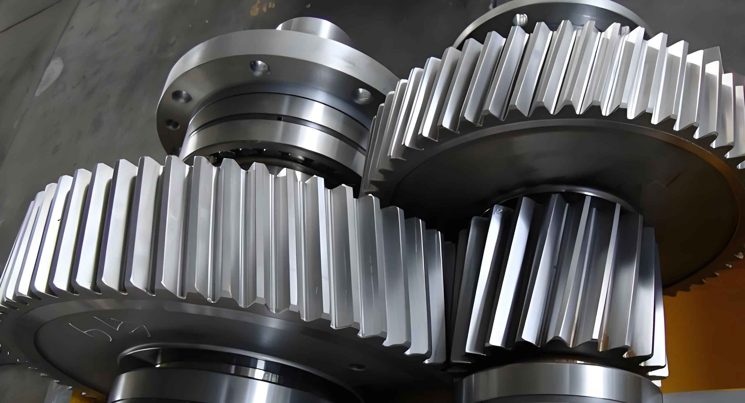
The dynamic performance of an EV is heavily influenced by the motor’s torque characteristics. For a PMSM, the vector control strategy with \(i_d = 0\) is widely used due to its simplicity and effectiveness. The mathematical model of the PMSM in the d-q rotating reference frame is given by the following equations. The voltage equations are:
$$ u_d = R_s i_d + p\psi_d – \omega_e \psi_q $$
$$ u_q = R_s i_q + p\psi_q + \omega_e \psi_d $$
where \(u_d\) and \(u_q\) are the d-axis and q-axis stator voltages, \(i_d\) and \(i_q\) are the corresponding currents, \(R_s\) is the stator resistance, \(p\) is the differential operator, \(\omega_e\) is the electrical angular velocity, and \(\psi_d\) and \(\psi_q\) are the flux linkages. The torque equation is:
$$ T_e = \frac{3}{2} p_n (\psi_d i_d – \psi_q i_q) = \frac{3}{2} p_n [\psi_f i_q + (L_d – L_q) i_d i_q] $$
Here, \(T_e\) is the electromagnetic torque, \(p_n\) is the number of pole pairs, \(\psi_f\) is the permanent magnet flux linkage, and \(L_d\) and \(L_q\) are the inductances. The mechanical motion equation is:
$$ J \frac{d\omega_m}{dt} = T_e – T_L – B\omega_m $$
where \(J\) is the combined inertia of the rotor and load, \(\omega_m\) is the mechanical angular velocity, \(T_L\) is the load torque, and \(B\) is the damping coefficient. The load torque \(T_L\) is derived from the vehicle dynamics, considering driving resistances such as rolling resistance, aerodynamic drag, gradient resistance, and acceleration resistance. The relationship is expressed as:
$$ T_L = \frac{\sum F \cdot r}{i_g i_0 \eta_T} $$
where \(\sum F\) is the total driving resistance, \(r\) is the wheel radius, \(i_g\) is the gear ratio of the transmission, \(i_0\) is the final drive ratio, and \(\eta_T\) is the mechanical efficiency. To simulate real-world conditions, we use the Urban Dynamometer Driving Schedule (UDDS) cycle, which represents typical city driving. The motor model is implemented in MATLAB/Simulink, and the simulation outputs the dynamic torque \(T_e\) over time. This torque profile, characterized by high-frequency fluctuations and sharp impacts, is then used as the input for the helical gear analysis.
The helical gear pair in the EV transmission is subjected to this dynamic torque. To compute the contact stresses on the helical gear teeth, we apply Hertzian contact theory. The maximum contact stress \(\sigma_H\) occurs at the pitch point of the pinion, which is the critical location for contact fatigue. For a helical gear, the contact stress can be calculated by first considering an equivalent spur gear based on the normal plane. The formula for the contact stress is:
$$ \sigma_H = \sqrt{ \frac{2T (1/R_1 + 1/R_2)}{d_1 \pi B \cos\alpha_n \cos\beta \left( \frac{1-\nu_1^2}{E_1} + \frac{1-\nu_2^2}{E_2} \right) } } $$
where \(T\) is the torque on the pinion (derived from the motor torque), \(R_1\) and \(R_2\) are the radii of curvature at the contact point, \(d_1\) is the pitch diameter of the pinion, \(B\) is the face width, \(\alpha_n\) is the normal pressure angle, \(\beta\) is the helix angle, \(\nu_1\) and \(\nu_2\) are Poisson’s ratios, and \(E_1\) and \(E_2\) are Young’s moduli for the pinion and gear, respectively. The radii of curvature are given by:
$$ R_1 = r_{b1} \tan\alpha $$
$$ R_2 = r_{b2} \tan\alpha $$
with \(r_{b1}\) and \(r_{b2}\) as the base circle radii and \(\alpha\) as the operating pressure angle. The parameters for the high-speed helical gear pair studied here are summarized in Table 1.
| Parameter | Symbol | Value |
|---|---|---|
| Normal module | \(m_n\) | 2.25 mm |
| Normal pressure angle | \(\alpha_n\) | 20° |
| Helix angle | \(\beta\) | 25° |
| Number of teeth (pinion/gear) | \(z_1 / z_2\) | 20 / 80 |
| Face width | \(B\) | 27 mm |
| Pitch diameter (pinion) | \(d_1\) | 45 mm |
| Base circle radius (pinion) | \(r_{b1}\) | 20 mm |
| Base circle radius (gear) | \(r_{b2}\) | 84 mm |
| Young’s modulus | \(E\) | 206 GPa |
| Poisson’s ratio | \(\nu\) | 0.3 |
Using the dynamic torque from the motor simulation, we compute the contact stress history over the UDDS cycle. This results in a stress spectrum that captures the time-varying loads on the helical gear. The stress spectrum is then processed for fatigue analysis. However, since the load on a single tooth is discontinuous per gear revolution, we rearrange the stress data to form a continuous load history for each tooth. This allows us to apply the rainflow counting method, which is a standard technique for extracting cycles from random load sequences. The rainflow counting yields the stress amplitude-mean-frequency relationship, as shown in Table 2, which summarizes the cycle counts for different stress levels.
| Stress Amplitude (MPa) | Mean Stress (MPa) | Number of Cycles |
|---|---|---|
| 50-100 | 450-550 | 1,200 |
| 100-150 | 500-600 | 850 |
| 150-200 | 550-650 | 420 |
| 200-250 | 600-700 | 180 |
| 250-300 | 650-750 | 75 |
| 300-350 | 700-800 | 30 |
For fatigue life prediction, we use the nominal stress approach based on S-N curves. The helical gear material’s S-N curve is modified to account for factors such as size effect, surface finish, and load type. The modified stress \(S_0\) is given by:
$$ S_0 = \sigma_0 \epsilon \beta C_L / K_T $$
where \(\sigma_0\) is the material S-N stress, \(\epsilon\) is the size factor, \(\beta\) is the surface factor, \(C_L\) is the load factor, and \(K_T\) is the stress concentration factor. We assume typical values: \(\epsilon = 0.86\), \(\beta = 0.90\), \(C_L = 0.85\), and \(K_T = 1.0\). Additionally, to consider loads below the fatigue limit, we apply the EM rule, which extends the S-N curve with the same slope. The modified P-S-N curve for a survival probability of 99% is derived, and the relationship between stress amplitude \(\sigma_a\) and cycles to failure \(N_i\) is expressed as:
$$ N_i = C \sigma_a^{-m} $$
where \(C\) and \(m\) are material constants. Since the stress cycles have non-zero mean stresses, we convert them to equivalent fully reversed cycles using the Goodman relation:
$$ \sigma_{eq} = \frac{\sigma_a}{1 – \frac{\sigma_m}{\sigma_u}} $$
where \(\sigma_{eq}\) is the equivalent stress amplitude, \(\sigma_a\) is the actual stress amplitude, \(\sigma_m\) is the mean stress, and \(\sigma_u\) is the ultimate tensile strength. The cumulative fatigue damage is calculated using Miner’s linear damage rule:
$$ D = \sum_{i=1}^{k} \frac{n_i}{N_i} $$
Here, \(n_i\) is the number of cycles at stress level \(i\), and \(N_i\) is the cycles to failure at that level. Failure occurs when \(D\) reaches 1. The total damage per UDDS cycle is computed by summing the damage from all stress cycles. Based on our analysis, the cumulative damage \(D\) for the helical gear in one UDDS cycle is found to be \(3.22 \times 10^{-5}\). Therefore, the fatigue life in terms of UDDS cycles is:
$$ T = \frac{1}{D} = \frac{1}{3.22 \times 10^{-5}} \approx 31,000 \text{ cycles} $$
This corresponds to a mileage of approximately 370,000 km for the EV, assuming the UDDS cycle represents typical urban driving. The results highlight the importance of considering dynamic motor loads in helical gear design for EVs. The helical gear’s performance under such conditions is critical for ensuring long-term reliability. To further elaborate, we can analyze the sensitivity of the helical gear life to various parameters. For instance, the helix angle \(\beta\) affects the contact stress through the cosine term in the denominator. A larger helix angle reduces the contact stress, potentially extending fatigue life. The relationship can be explored using the following equation derived from the contact stress formula:
$$ \sigma_H \propto \frac{1}{\sqrt{\cos\beta}} $$
Thus, optimizing the helix angle is key for helical gear applications in EVs. Additionally, the dynamic torque from the motor includes high-frequency components that may excite resonant frequencies in the helical gear system. The natural frequency of a helical gear pair can be estimated using:
$$ f_n = \frac{1}{2\pi} \sqrt{\frac{k_{mesh}}{m_{eq}}} $$
where \(k_{mesh}\) is the mesh stiffness and \(m_{eq}\) is the equivalent mass. The mesh stiffness for a helical gear varies with the contact ratio and helix angle. For a helical gear, the total contact ratio is the sum of the transverse contact ratio and the overlap ratio:
$$ \epsilon_{\gamma} = \epsilon_{\alpha} + \epsilon_{\beta} $$
with \(\epsilon_{\alpha} = \frac{\sqrt{r_{a1}^2 – r_{b1}^2} + \sqrt{r_{a2}^2 – r_{b2}^2} – a \sin\alpha_t}{\pi m_t \cos\alpha_t}\) and \(\epsilon_{\beta} = \frac{B \sin\beta}{\pi m_n}\), where \(r_a\) is the addendum radius, \(a\) is the center distance, \(m_t\) is the transverse module, and \(\alpha_t\) is the transverse pressure angle. The dynamic load factor \(K_v\) can be incorporated to account for internal excitations, but in this study, we focus on the quasi-static approach for simplicity.
Another aspect is the thermal effects on the helical gear due to high-speed operation. The temperature rise can reduce material strength and affect lubrication. The flash temperature \(\theta_{flash}\) at the contact can be approximated by:
$$ \theta_{flash} = \frac{\mu W v}{4b k} $$
where \(\mu\) is the coefficient of friction, \(W\) is the load per unit width, \(v\) is the sliding velocity, \(b\) is the semi-width of the contact area, and \(k\) is the thermal conductivity. For helical gears, the sliding velocity varies along the tooth profile, and the helix angle influences the load distribution. However, for fatigue life prediction, we assume isothermal conditions and focus on mechanical stresses.
The reliability of the helical gear can also be assessed using probabilistic methods. Given the scatter in material properties and loads, the probability of survival \(P_s\) can be related to the stress and life through Weibull distribution. The Weibull equation for fatigue life is:
$$ P_s = \exp\left[-\left(\frac{N}{N_0}\right)^b\right] $$
where \(N_0\) is the characteristic life and \(b\) is the shape parameter. Combining this with the S-N curve, we can predict life with a certain confidence level. In our case, the 99% survival probability is already considered in the P-S-N curve.
In summary, this study presents a comprehensive framework for analyzing dynamic loads and predicting fatigue life for high-speed helical gears in EVs. The methodology integrates motor dynamics, gear contact mechanics, and fatigue theory. The helical gear is central to this analysis, and its design parameters significantly impact the results. Future work could include experimental validation, multi-body dynamic simulations, and consideration of lubrication effects. Nonetheless, the current approach provides a practical tool for engineers to optimize helical gear systems in electric vehicles, ensuring durability and performance under real-world driving conditions.
To conclude, the dynamic behavior of EV motors imposes challenging loading conditions on transmission gears, particularly helical gears. By leveraging motor dynamic models and fatigue analysis, we can accurately compute stresses and predict life, thereby enhancing the design and reliability of EV drivetrains. The repeated emphasis on helical gear throughout this study underscores its importance in modern electric vehicle technology.