
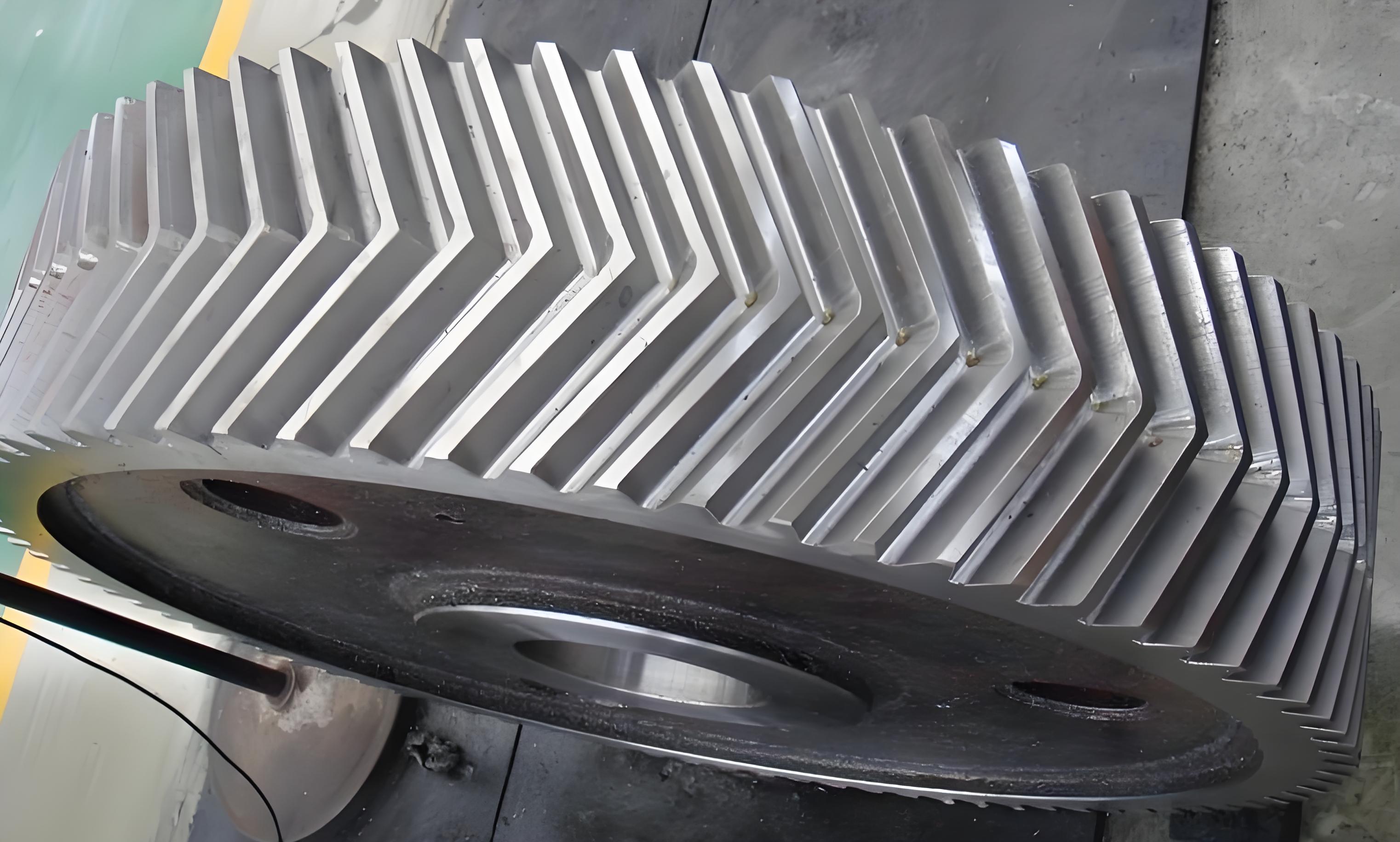
Gear transmission systems, particularly herringbone gears, are renowned for their smooth operation, high load capacity, and excellent axial force balancing properties. These advantages make them indispensable in high-performance applications such as aerospace propulsion, marine drives, and precision machine tools. The dynamic characteristics of these systems are not solely determined by their ideal design parameters; they are significantly influenced by the inevitable manufacturing and assembly errors inherent in all mechanical components. A comprehensive and rational consideration of these errors within the system’s dynamic model is fundamental for accurately analyzing their impact on performance, which is crucial for vibration reduction, noise control, and reliability enhancement. Traditional dynamic models often consider errors in isolation, such as gear tooth deviations or bearing clearances, but lack a holistic approach to account for the spatial accumulation of errors from multiple components like housings, shafts, and bearings across the entire assembly chain.
This paper addresses this gap by proposing an integrated dynamic model for a herringbone gear transmission system that explicitly incorporates the cumulative effects of system-wide manufacturing and assembly errors. The methodology synergistically couples a finite-element-based dynamic model of the gear-rotor-bearing system with a three-dimensional tolerance analysis model, specifically the Jacobian-Torsor model. The Jacobian-Torsor model is adept at representing and propagating the small displacements (translational and rotational errors) of features within an assembly’s tolerance zones. This coupling allows for the first-principles calculation of the resultant posture errors (cumulative errors) at the pinion and gear locations, which are then introduced as excitation sources into the dynamic equations of motion. The integrated model enables a direct link between the geometric tolerances specified during the design phase and the resulting dynamic response of the herringbone gear system.
Establishing the Cumulative Error Model for the Herringbone Gear System
The system under study is a single-stage, parallel-axis herringbone gear reducer. The assembly consists of a gearbox housing, a high-speed pinion shaft, a low-speed gear shaft, the large low-speed herringbone gear, and supporting bearings. The dynamic excitation and vibration response are critically dependent on the relative positional and orientational deviations of the mating herringbone gears, which arise from the accumulation of errors from all components in the load path. The basic parameters of the herringbone gear pair are summarized in Table 1.
| Parameter | Pinion | Gear |
|---|---|---|
| Number of Teeth, $z$ | 23 | 46 |
| Normal Module, $m_n$ (mm) | 5 | 5 |
| Normal Pressure Angle, $\alpha_n$ (°) | 20 | 20 |
| Helix Angle, $\beta$ (°) | 24.784 | 24.784 |
| Face Width (per helix), $B$ (mm) | 50 | 50 |
| Pinion Speed, $n$ (rpm) | 1000 | – |
| Input Torque, $T$ (N·m) | 432 | – |
Table 1: Basic parameters of the herringbone gear pair.
Dimensional Chain and Tolerance Representation
The first step involves constructing a dimensional chain transfer diagram that maps all relevant error sources (Functional Elements, FEs) from the mounting interfaces to the functional requirements (FRs), which are defined as the cumulative posture errors at the centers of the pinion and the gear. Errors are categorized as Internal Functional Elements (IFEs, between features on the same part), Contact Functional Elements (CFEs, between mating parts), and, after processing, Parallel Functional Elements (PFEs, for parallel assembly paths). The tolerance values associated with key FEs, such as housing bore location/coaxiality, bearing fit clearances, and gear runout, are listed in Table 2.
| FE Symbol | Description | Tolerance Value (mm) |
|---|---|---|
| IFE1 | Position of Bore 1 Axis, Parallelism | 0.02, 0.015 |
| IFE2 | Coaxiality of Bore 2 Axis | 0.02 |
| IFE3 | Coaxiality of Bore 3 Axis | 0.02 |
| IFE4 | Position of Bore 4 Axis, Parallelism | 0.02, 0.015 |
| IFE5 | Pinion Radial Runout | 0.02 |
| IFE6 | Gear Radial Runout | 0.02 |
| CFE1 | Bore 1 & Bearing Outer Ring Fit | Size: (-0.021,+0.004), Cylindricity: 0.008, etc. |
| CFE9 | Face Runout at Gear-Shaft Fit | 0.015 |
Table 2: Tolerances of key functional elements in the assembly.
Each FE’s potential variation within its tolerance zone is described by a small displacement torsor $T$, which contains three translational ($u, v, w$) and three rotational ($\alpha, \beta, \gamma$) components along/about the local coordinate axes:
$$ T = [u, v, w, \alpha, \beta, \gamma]^T \quad \text{s.t.} \quad \underline{u} \leq u \leq \overline{u}, \ldots, \underline{\gamma} \leq \gamma \leq \overline{\gamma} $$
The bounds for each component are derived from the tolerance specifications. For example, the torsor for IFE1, constrained by both position and parallelism tolerances, is derived as the intersection of the individual tolerance domains. Using a Monte Carlo sampling method within these bounds, the statistical ranges for the torsor parameters of each FE are determined, as exemplified for a subset in Table 3.
| FE Symbol | Torsor Model $T$ (approximate range) |
|---|---|
| IFE1 | $[\pm9.43\times10^{-3}, \pm9.43\times10^{-3}, 0, \pm2.09\times10^{-4}, \pm2.09\times10^{-4}, 0]$ |
| IFE5 | $[\pm6.99\times10^{-3}, \pm6.99\times10^{-3}, 0, \pm8.4\times10^{-5}, \pm8.4\times10^{-5}, 0]$ |
| CFE9 | $[0, 0, \pm7.09\times10^{-3}, \pm9.08\times10^{-5}, 0, \pm9.08\times10^{-5}]$ |
Table 3: Torsor models for selected functional elements.
Error Propagation using the Jacobian-Torsor Model
The propagation of these small deviations from each FE to the FR is calculated using the Jacobian-Torsor model. The Jacobian matrix $J_{FE_i}$ for an FE describes how its small displacement affects the FR based on the relative position and orientation between the FE’s local frame and the FR’s frame. For the coordinate systems defined in this analysis, the Jacobian typically takes the form:
$$ J_{FE_i} =
\begin{bmatrix}
1 & 0 & 0 & 0 & \Delta z & 0 \\
0 & 1 & 0 & -\Delta z & 0 & 0 \\
0 & 0 & 1 & 0 & 0 & 0 \\
0 & 0 & 0 & 1 & 0 & 0 \\
0 & 0 & 0 & 0 & 1 & 0 \\
0 & 0 & 0 & 0 & 0 & 1
\end{bmatrix}, \quad \text{where } \Delta z = z_{FE_i} – z_{FR} $$
The cumulative torsor $T_{FR}$ at the functional requirement (e.g., the pinion location) is obtained by summing the contributions of all FEs in the chain:
$$ T_{FR} = \sum_{i} (J_{FE_i} \cdot T_{FE_i}) $$
For parallel assembly paths, such as the shaft defined by two bearing locations, a homogenization method is applied. Points $M_0$ and $M_1$ are defined on the nominal high-speed and low-speed shaft axes, respectively. The equivalent torsors for the parallel paths, $T_{PFE1}$ and $T_{PFE2}$, representing the high-speed and low-speed shaft errors, are calculated. Finally, the cumulative error torsors at the pinion ($FR1$) and gear ($FR2$) centers are computed as:
$$ T_{FR1} = J_{PFE1} \cdot T_{PFE1} + J_{IFE5} \cdot T_{IFE5} $$
$$ T_{FR2} = J_{PFE2} \cdot T_{PFE2} + J_{CFE9} \cdot T_{CFE9} + J_{IFE6} \cdot T_{IFE6} $$
These torsors, $FR1 = [u_1, v_1, w_1, \alpha_1, \beta_1, \gamma_1]$ and $FR2 = [u_2, v_2, w_2, \alpha_2, \beta_2, \gamma_2]$, represent the complete spatial deviation of the herringbone gears from their ideal positions and orientations due to all considered system errors.
Development of the System Dynamic Model
Baseline Dynamic Model Without Cumulative Errors
A finite element method (FEM) based dynamic model is established for the herringbone gear transmission system. The herringbone gear is modeled as two helical gear halves connected by a flexible shaft segment. The system model comprises shaft elements, bearing support elements, and gear mesh elements, totaling 34 nodes with 136 degrees of freedom (three translations and one torsion about the shaft axis per node).
The left and right helical gear pairs have opposite hand of helix. The projection vector $V_k$ ($k=l, r$ for left/right) that maps the nodal displacements onto the line of action for each pair is:
$$ V_k = [\pm\cos\beta_b \sin\phi, \pm\cos\beta_b \cos\phi, \sin\beta_b, \pm r_{p}\cos\beta_b, \mp\cos\beta_b \sin\phi, \mp\cos\beta_b \cos\phi, -\sin\beta_b, \mp r_{g}\cos\beta_b] $$
where $\beta_b$ is the base helix angle, $\phi$ is the angle from the y-axis to the plane of action, and $r_p$, $r_g$ are the base circle radii.
The relative dynamic transmission error $\delta_{m,k}$ along the line of action for gear pair $k$ is:
$$ \delta_{m,k} = V_k \cdot q_{m,k} – e_{m,k}(t) $$
where $q_{m,k}$ is the displacement vector of the mating gear nodes and $e_{m,k}(t)$ is the static transmission error excitation. The equation of motion for a mesh element is:
$$ M_m \ddot{q}_{m,k} + C_m \dot{q}_{m,k} + K_m \delta_{m,k} = 0 $$
with $C_m = c_m V_k^T V_k$ and $K_m = k_m(t) V_k^T V_k$, where $c_m$ is the mesh damping and $k_m(t)$ is the time-varying mesh stiffness. Assembling all element matrices yields the global system equation:
$$ M_{all} \ddot{x} + C_{all} \dot{x} + K_{all} x = F_{all} $$
Enhanced Dynamic Model Integrating Cumulative Errors
The cumulative error torsors $FR1$ and $FR2$ directly alter the spatial relationship between the mating herringbone gears. This affects the dynamic model in two primary ways: 1) introducing a quasi-static displacement excitation, and 2) modifying the gear mesh parameters (stiffness and unloaded transmission error).
The posture change defined by $FRj$ ($j=1,2$) is represented by a homogeneous transformation matrix $M_{FRj}$ derived from its torsor components. This matrix transforms the coordinates of any point on the gear from its nominal to its actual position. The additional displacement $E_k$ of the gear centers along the line of action due to cumulative errors is:
$$ E_k = V_k \cdot [X_{pk}, Y_{pk}, Z_{pk}, 0, X_{gk}, Y_{gk}, Z_{gk}, 0]^T $$
where $(X_{pk}, Y_{pk}, Z_{pk})$ and $(X_{gk}, Y_{gk}, Z_{gk})$ are the actual coordinates of the pinion and gear centers for helix $k$, obtained by transforming their nominal coordinates using $M_{FR1}$ and $M_{FR2}$.
Furthermore, the cumulative errors alter the initial gaps between potential tooth contact points. For a discrete point $P_n$ on the tooth surface, its coordinate deviation $\Delta r_{jn}$ in the gear’s local frame due to $FRj$ is:
$$ [\Delta x_{jn}, \Delta y_{jn}, \Delta z_{jn}, 1]^T = M_{FRj} \cdot [x_{jn}, y_{jn}, z_{jn}, 1]^T – [x_{jn}, y_{jn}, z_{jn}, 1]^T $$
The resultant change in the initial separation $\epsilon_n$ at point $P_n$ is $\epsilon_n = \sum_{j=1}^{2} \Delta r_{jn} \cdot n_{jn}$, where $n_{jn}$ is the surface normal. This modified gap is incorporated into the loaded tooth contact analysis to compute the updated time-varying mesh stiffness $k’_m(t)$ and loaded static transmission error $e’_m(t)$ for each helical pair under the erroneous posture.
The enhanced relative deformation for the dynamic model becomes:
$$ X_{m,k} = V_k \cdot q_{m,k} – e’_{m,k}(t) – E_k $$
Substituting $X_{m,k}$ for $\delta_{m,k}$ and using $k’_m(t)$ in the mesh stiffness matrix $K_m$ yields the final system equations of motion that fully account for the system’s cumulative manufacturing and assembly errors. This integrated model forms the basis for all subsequent dynamic analyses.
Analysis of System Dynamic Characteristics
Dynamic simulations are performed under the operating conditions specified in Table 1. The dynamic load factor $Kd_k$, which quantifies the severity of dynamic loading relative to the nominal load, is a key performance indicator. It is calculated for each helical pair as:
$$ Kd_k = \frac{\max(F_k(t))}{F_n} $$
where $F_k(t)$ is the dynamic mesh force and $F_n$ is the nominal static mesh force.
Influence of Individual Error Components
Seventeen independent error parameters (e.g., $X1$: translational error of PFE1 along y, $X2$: rotational error of PFE1 about x) are identified from the torsor models. The effect of varying each parameter individually across its tolerance range on the dynamic load factors is analyzed. The results, shown graphically, reveal that parameters associated with the parallel path elements—specifically the translational ($X1$, $X8$) and rotational ($X2$, $X9$) errors of the high-speed and low-speed shaft lines—have the most pronounced influence on the dynamic load factors of both the left and right herringbone gear pairs. Other parameters related to individual gear runout or bearing fits show a comparatively minor effect. This sensitivity analysis highlights that in tolerance design, controlling the errors contributing to the shaft line posture (e.g., housing bore coaxiality for bore 2, which influences $PFE2$) is paramount for optimizing dynamic performance.
Influence of Coupled Errors on Dynamic Response
In reality, all errors act simultaneously. Five different error combination scenarios are generated via Latin Hypercube Sampling within the tolerances ranges. The mesh excitations—time-varying stiffness $k’_m(t)$ and transmission error $e’_m(t)$—are recalculated for each scenario. A sample of the error combinations is shown in Table 4.
| Scenario | $X1$ (mm) | $X2$ (rad) | $X8$ (mm) | $X9$ (rad) |
|---|---|---|---|---|
| 1 | 0.0020 | 3.68e-4 | 0.0407 | -3.12e-4 |
| 2 | 0.0247 | -3.64e-4 | -0.0321 | 2.59e-4 |
| 3 | 0.0069 | -5.01e-5 | 0.0233 | -1.07e-4 |
Table 4: Example error parameter values for different combination scenarios.
The analysis reveals that coupled errors break the symmetry of the herringbone gear. The mesh stiffness curves for the left and right helical pairs become distinct, though their mean values change only slightly (<4%). The primary impact is on the transmission error, whose mean value and fluctuation amplitude increase under most error combinations. The motion trajectories of the gear centers in the transverse plane are also affected, showing expanded or contracted orbits compared to the error-free case.
The dynamic mesh forces and corresponding load factors for the left and right sides are no longer identical, indicating a loss of perfect load sharing. Crucially, as shown in Figure 10(c) of the simulated results, the dynamic load factors for some error combinations (e.g., Scenarios 1, 3, and 4) are actually lower than the baseline error-free value of 1.221. This demonstrates that the coupled effect of multiple system errors is not always detrimental; certain combinations can, by chance or design, interact in a way that mitigates dynamic excitation and improves the overall dynamic performance of the herringbone gear transmission system.
Conclusion
This paper successfully developed and demonstrated an integrated modeling framework for analyzing the dynamics of herringbone gear transmission systems under the influence of system-wide cumulative manufacturing and assembly errors. The core achievement is the coupling of a finite-element dynamic model with a Jacobian-Torsor based three-dimensional tolerance analysis model. This approach allows for a comprehensive and physically consistent incorporation of spatial error accumulation from components like the housing, shafts, and bearings into the dynamic simulation.
The key findings from the analysis are: 1) Among all individual error sources, the translational and rotational posture errors of the high-speed and low-speed shaft lines (represented by parameters like $X1$, $X2$, $X8$, $X9$) have the most significant impact on the system’s dynamic load factors. 2) These critical error parameters originate from the synthesis of tolerances on associated features (e.g., housing bore coaxiality), providing a direct target for tolerance design optimization aimed at vibration reduction. 3) The dynamic response under coupled errors shows that the left and right sides of the herringbone gear experience different dynamic loads, breaking ideal load sharing. 4) Importantly, the coupled effect of multiple errors is not purely additive; specific combinations can lead to a dynamic load factor lower than that of the nominal error-free system, suggesting potential avenues for robust design or selective assembly to harness favorable error interactions.
This work establishes a vital link between the geometric domain of tolerance design and the functional domain of dynamic performance for herringbone gear systems. The proposed model serves as a foundation for future research into tolerance allocation strategies, robustness optimization, and performance prediction that account for real-world manufacturing variations.