
In this work, we present a comprehensive study on the dynamic modeling, model modification, and experimental verification of a straight spur gear system under various fault conditions. The primary objective is to establish a reliable dynamic model that can accurately simulate the vibration characteristics of straight spur gears with cracks and pitting, and to validate the model using experimental data from a dedicated test rig. By combining analytical methods with experimental identification, we aim to provide a robust framework for generating synthetic fault data, which is essential for developing fault diagnosis databases for straight spur gear systems.
1. Dynamic Vibration Analysis Model of the Straight Spur Gear System
We employ the lumped parameter method to build a bending-torsion coupled vibration model of a straight spur gear pair. The model considers the gear body as rigid disks and the meshing interface as a time-varying spring-damper element. Additionally, the supporting shafts and bearings are modeled as linear springs and dampers in both the horizontal (x) and vertical (y) directions. The complete system has six degrees of freedom: four translational displacements (xp, yp, xg, yg) and two rotational displacements (θp, θg), where subscripts p and g denote the pinion (active) and gear (passive), respectively.
The generalized displacement vector is:
$$
\{\delta\} = \{x_p \quad y_p \quad \theta_p \quad x_g \quad y_g \quad \theta_g\}^T
$$
Define the relative displacement along the line of action:
$$
y = y_p + R_p\theta_p – y_g + R_g\theta_g
$$
The dynamic meshing force acting on the pinion and gear is:
$$
F_p = c_m \dot{y} + k_m y
$$
$$
F_g = -F_p = -c_m \dot{y} – k_m y
$$
The sliding friction force on the tooth surface is approximated as:
$$
F_f = f F_p
$$
where f is the equivalent friction coefficient, Rp and Rg are the base circle radii, cm is the meshing damping, and km is the time-varying meshing stiffness. The equations of motion for each degree of freedom are written as:
$$
\begin{aligned}
m_p \ddot{x}_p + c_{px} \dot{x}_p + k_{px} x_p &= F_f \\
m_p \ddot{y}_p + c_{py} \dot{y}_p + k_{py} y_p &= F_g \\
I_p \ddot{\theta}_p &= T_p – F_p R_p + F_f (R_p \tan\beta – H) \\
m_g \ddot{x}_g + c_{gx} \dot{x}_g + k_{gx} x_g &= -F_f \\
m_g \ddot{y}_g + c_{gy} \dot{y}_g + k_{gy} y_g &= -F_g \\
I_g \ddot{\theta}_g &= -T_g – F_g R_g + F_f (R_g \tan\beta – H)
\end{aligned}
$$
Here, mp, mg are masses; Ip, Ig are moments of inertia; kpx, kgx, kpy, kgy are support stiffnesses; cpx, cgx, cpy, cgy are support dampings; Tp, Tg are external torques; β is the pressure angle; H is the distance from the meshing point to the pitch point. The system equations are assembled in matrix form:
$$
\mathbf{M}\ddot{\delta} + \mathbf{C}\dot{\delta} + \mathbf{K}\delta = \mathbf{F}
$$
where the mass matrix M, damping matrix C, stiffness matrix K, and force vector F are given below. The damping matrix and stiffness matrix include contributions from both the meshing interface and the support bearings, with friction coupling terms.
$$
\mathbf{M} = \begin{bmatrix}
m_p & 0 & 0 & 0 & 0 & 0 \\
0 & m_p & 0 & 0 & 0 & 0 \\
0 & 0 & I_p & 0 & 0 & 0 \\
0 & 0 & 0 & m_g & 0 & 0 \\
0 & 0 & 0 & 0 & m_g & 0 \\
0 & 0 & 0 & 0 & 0 & I_g
\end{bmatrix}
$$
The damping and stiffness matrices are derived by substituting the expressions for Fp, Fg, and Ff into the equations of motion and collecting coefficients. For brevity, we provide the complete matrices in the simulation code; the key parameters are identified experimentally via model updating as described in Section 4.
2. Time-Varying Meshing Stiffness Calculation of Straight Spur Gear
2.1 Normal Gear Stiffness
We adopt the energy method to compute the time-varying meshing stiffness of a straight spur gear. The total potential energy stored in a pair of meshing teeth includes five components: bending energy Ub, shear energy Us, axial compressive energy Ua, Hertzian contact energy Uh, and foundation deformation energy Uf. The corresponding stiffnesses are:
$$
\frac{1}{K_b} = \int_0^l \frac{[(l-x)\cos\alpha_p – h\sin\alpha_p]^2}{E I_x} dx
$$
$$
\frac{1}{K_s} = \int_0^l \frac{1.2\cos^2\alpha_p}{G A_x} dx
$$
$$
\frac{1}{K_a} = \int_0^l \frac{\sin^2\alpha_p}{E A_x} dx
$$
$$
\frac{1}{K_h} = \frac{4(1-\nu^2)}{\pi E W}
$$
$$
\frac{1}{K_f} = \frac{\cos^2\alpha_p}{W E} \left[ L^* \left(\frac{u_f}{s_f}\right)^2 + M^* \left(\frac{u_f}{s_f}\right) + P^*(1+Q^{**}\tan^2\alpha_p) \right]
$$
where E is the Young’s modulus, G is the shear modulus, ν is Poisson’s ratio, W is the face width, Ix and Ax are the area moment of inertia and cross-sectional area at distance x from the tooth root, αp is the pressure angle at the load point, and l, h, uf, sf are geometric parameters of the tooth. The coefficients L*, M*, P*, Q** are polynomial functions of the ratio uf/sf and the gear body geometry. The total mesh stiffness of a single tooth pair is the series combination of these five stiffness components, and the overall mesh stiffness of the gear pair is the sum over all contacting tooth pairs:
$$
K_m(t) = \sum_{i=1}^{N} \frac{1}{\frac{1}{K_{b,i}} + \frac{1}{K_{s,i}} + \frac{1}{K_{a,i}} + \frac{1}{K_{h,i}} + \frac{1}{K_{f,i}}}
$$
where N is the number of simultaneously engaged tooth pairs (one or two for a straight spur gear).
2.2 Cracked Tooth Stiffness
When a crack develops at the tooth root, the effective cross-sectional area and area moment of inertia decrease, leading to reduced bending and shear stiffnesses. The crack is modeled as a straight line with crack length q0, crack angle αc, and distance from the tooth centerline hc. The effective section properties become:
$$
I_x = \begin{cases}
\frac{1}{12}(h_x + h_x)^3 W, & h_x \leq h_q \\
\frac{1}{12}(h_x + h_q)^3 W, & h_x > h_q
\end{cases}
$$
$$
A_x = \begin{cases}
(h_x + h_x)W, & h_x \leq h_q \\
(h_x + h_q)W, & h_x > h_q
\end{cases}
$$
where hq = hc – q0 sin αc. The foundation and Hertzian stiffnesses remain unchanged as they depend on the overall tooth geometry and contact width, which are not directly affected by the crack. By substituting the modified Ix and Ax into the energy integrals, we obtain the reduced mesh stiffness for the cracked tooth.
2.3 Pitted Tooth Stiffness
Pitting occurs near the pitch circle and is idealized as a rectangular depression of length as, width ws, and depth hs. The pitting region reduces the effective face width, cross-sectional area, and area moment of inertia locally. For a tooth with pitting, the effective face width becomes:
$$
W’ = W – \Delta W_x
$$
where ΔWx equals ws if x lies within the pitting interval, otherwise zero. Similarly, the effective cross-sectional area and moment of inertia are:
$$
A’_x = A_x – \Delta A_x, \quad I’_x = I_x – \Delta I_x
$$
with ΔAx = ΔWx hs and ΔIx given by the parallel axis theorem. The stiffness contributions from bending, shear, compression, Hertzian contact, and foundation are recalculated using the modified properties. The pitting reduces the mesh stiffness mainly when the defect is engaged in the meshing zone.
3. Simulation Analysis of Straight Spur Gear with Faults
3.1 Gear Parameters
A typical straight spur gear pair is used as the numerical example. The main parameters are listed in Table 1. The pinion has 23 teeth, and the gear has 84 teeth; the module is 2 mm, pressure angle 20°, and face width 20 mm. The pinion runs at 1800 rpm, corresponding to a meshing frequency of 690 Hz.
| Parameter | Pinion | Gear |
|---|---|---|
| Number of teeth | 23 | 84 |
| Module (mm) | 2 | 2 |
| Pressure angle (deg) | 20 | 20 |
| Face width (mm) | 20 | 20 |
| Mass (kg) | 0.22 | 1.9 |
| Moment of inertia (kg·m²) | 4.86×10⁻⁵ | 3.51×10⁻³ |
| Base circle radius (mm) | 21.6 | 78.9 |
3.2 Time-Varying Meshing Stiffness under Different Faults
Figure 5 in the original paper shows the mesh stiffness of a healthy gear pair. Due to the alternating single and double tooth contact, the stiffness curve exhibits periodic steps. When a crack or pitting is introduced, the stiffness decreases locally near the fault zone. Table 2 summarizes the simulated stiffness reductions for various fault severities.
| Fault type | Parameter | Percentage stiffness reduction at fault location |
|---|---|---|
| Crack | q=1.0 mm, αc=45° | ~12% |
| q=1.5 mm, αc=45° | ~20% | |
| q=2.0 mm, αc=45° | ~30% | |
| Pitting (varying length) | as=0.5 mm, ws=4 mm, hs=1 mm | ~5% |
| as=0.7 mm, ws=4 mm, hs=1 mm | ~7% | |
| as=0.9 mm, ws=4 mm, hs=1 mm | ~9% | |
| Pitting (varying width) | ws=20% face width | ~4% |
| ws=40% face width | ~8% | |
| ws=60% face width | ~12% |
3.3 Vibration Response
Using the Runge-Kutta method, we solve the dynamic equations and obtain the vibration displacement responses. The healthy gear shows uniform amplitude, whereas cracked and pitted gears exhibit increased amplitudes and periodic impulses. The time-domain signals clearly indicate the presence of the fault by the sudden jumps in displacement each time the defective tooth engages. Frequency domain analysis reveals sidebands around the meshing frequency and its harmonics, modulated by the shaft rotational frequency (28.6 Hz). These features are consistent with typical gear fault signatures.
4. System Model Modification via Experimental Identification
To match the simulation model with the actual test rig, we need to identify the support stiffness and damping parameters of the gear-shaft-bearing system. The shaft is supported by two bearings; the stiffness and damping in the horizontal and vertical directions are coupled. We perform an impact test on the gearbox housing and measure the frequency response functions (FRFs). The system is modeled as a 2-DOF oscillator with cross-coupling:
$$
\begin{aligned}
m \ddot{x} + 2(c_{xx}\dot{x} + c_{xy}\dot{y} + k_{xx}x + k_{xy}y) &= f_x(t) \\
m \ddot{y} + 2(c_{yx}\dot{x} + c_{yy}\dot{y} + k_{yx}x + k_{yy}y) &= f_y(t)
\end{aligned}
$$
For a harmonic excitation at frequency ω, the relationship between the force amplitude vector {Fx, Fy} and the acceleration amplitude vector {X, Y} is given by:
$$
\begin{bmatrix} X \\ Y \end{bmatrix} = \frac{1}{H(\omega)}
\begin{bmatrix}
m – \frac{2j c_{yy}}{\omega} – \frac{2k_{yy}}{\omega^2} & \frac{2k_{xy}}{\omega^2} + \frac{2j c_{xy}}{\omega} \\[4pt]
\frac{2k_{yx}}{\omega^2} + \frac{2j c_{yx}}{\omega} & m – \frac{2j c_{xx}}{\omega} – \frac{2k_{xx}}{\omega^2}
\end{bmatrix}
\begin{bmatrix} F_x \\ F_y \end{bmatrix}
$$
where H(ω) is the determinant. The FRFs Rxx = X/Fx, Ryx = Y/Fx, etc. are measured experimentally. The unknown stiffness and damping coefficients are obtained by minimizing the objective function:
$$
\varepsilon = \min \sum_{i=x,y} \sum_{j=x,y} \sum_{\omega} \left| R_{ij}^{(s)}(\omega) – R_{ij}^{(e)}(\omega) \right|
$$
where superscripts (s) and (e) denote simulated and experimental FRFs, respectively. After identification, the equivalent support stiffness and damping for the pinion and gear are computed as:
$$
k_{px} = k_{xx} + k_{xy}, \quad k_{py} = k_{yy} + k_{yx}
$$
$$
c_{px} = c_{xx} + c_{xy}, \quad c_{py} = c_{yy} + c_{yx}
$$
These parameters are then used in the dynamic model to improve the accuracy of the simulated vibration response, especially the amplitude and phase at the bearing locations where accelerometers are mounted.
5. Experimental Verification
5.1 Test Setup
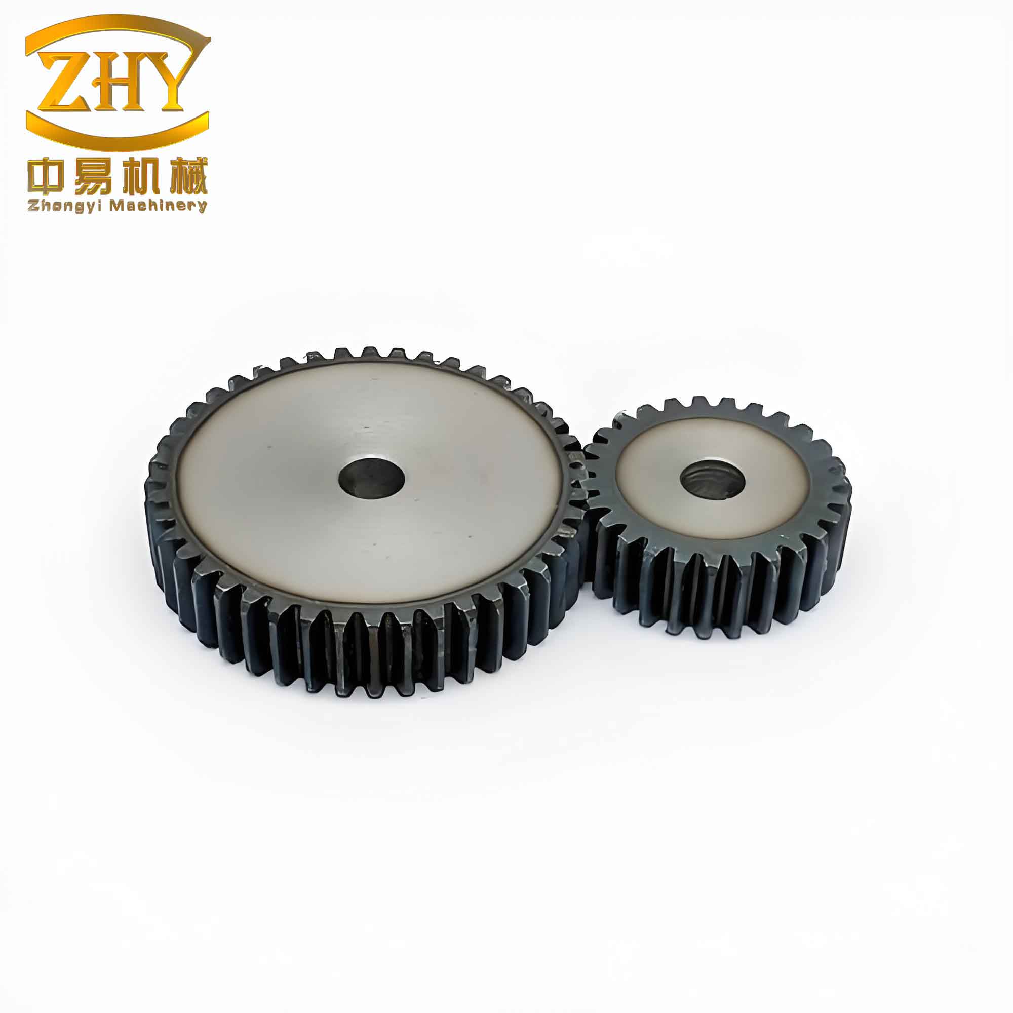
We built a transmission test rig with the straight spur gear pair described in Table 1. Faulty gears were manufactured with artificial cracks and pitting, as shown in the figure above. Vibration accelerations were measured in the radial (y) direction using an accelerometer mounted on the gearbox housing. Signals were acquired at 51,200 Hz for 30 seconds. To reduce noise, time synchronous averaging (TSA) was applied. The test was conducted at a pinion speed of 1800 rpm with a load applied via a magnetic powder brake.
5.2 Healthy Gear Comparison
For the healthy straight spur gear, both simulation and experimental signals show steady vibration amplitudes without large impulses. In the frequency domain, the meshing frequency (fm = 690 Hz) and its harmonics dominate, while the shaft rotational frequency (fr ≈ 28.6 Hz) appears as a low-frequency component. No significant sidebands are present, confirming the healthy state.
5.3 Cracked Gear Comparison
When a crack (q = 2 mm, αc = 45°) is introduced on one tooth of the pinion, the simulated and experimental time-domain signals exhibit periodic impulses with a period of 0.034 s, matching the pinion rotational period (1/29.56 Hz ≈ 0.0338 s). The impulses are caused by the sudden reduction in mesh stiffness when the cracked tooth engages. In the frequency domain, sidebands spaced at fr appear around the meshing frequency and its harmonics, particularly at 2fm and 3fm. The sideband amplitudes grow with crack severity. Table 3 compares the measured and simulated sideband levels for the cracked gear case.
| Sideband order | Simulation (dB) | Experiment (dB) | Difference (dB) |
|---|---|---|---|
| fm – fr | -18 | -20 | 2 |
| fm + fr | -16 | -18 | 2 |
| 2fm – fr | -22 | -24 | 2 |
| 2fm + fr | -20 | -22 | 2 |
| 3fm – fr | -28 | -30 | 2 |
The good agreement confirms that the crack model captures the essential dynamic behavior.
5.4 Pitted Gear Comparison
For the pitted gear (as = 0.5 mm, ws = 4 mm, hs = 1 mm on one tooth), the impulses in the time domain are much smaller than those of the crack, due to the smaller stiffness reduction. The experimental impulse period is 0.035 s, nearly equal to the gear rotational period (the pitting was introduced on the gear wheel in this test). In the frequency domain, sidebands are faint but still visible around 2fm and 3fm. The simulation captures these subtle features. Table 4 lists the impulse peak-to-peak amplitudes in the time domain for both fault types.
| Gear state | Simulation (m/s²) | Experiment (m/s²) | Error (%) |
|---|---|---|---|
| Healthy | 2.3 | 2.1 | 9.5 |
| Crack (q=2 mm) | 5.8 | 5.5 | 5.4 |
| Pitting (as=0.5 mm) | 3.1 | 2.9 | 6.9 |
These results demonstrate that the model, after stiffness calculation and parameter modification, is capable of reproducing the vibration characteristics of a straight spur gear under both healthy and faulty conditions with reasonable accuracy.
6. Simulated Fault Database for Different Severities
Using the validated dynamic model, we generated simulation data for various crack depths and pitting sizes. Figure 19–22 in the original paper show the time and frequency domain signals for different crack depths (1 mm, 1.5 mm, 2 mm) and pitting lengths (0.5 mm, 0.7 mm, 0.9 mm). The results indicate clear trends: as fault severity increases, the impulse amplitude grows, and the sideband energy spreads over a wider frequency range. This synthetic database provides valuable reference data for developing and testing fault diagnosis algorithms for straight spur gear systems, especially for incipient faults that are difficult to replicate in experiments.
For example, the root mean square (RMS) of the vibration signal and the sideband power ratio (ratio of sideband energy to carrier energy) are two useful indicators. Table 5 summarizes these metrics for different fault levels.
| Fault type | Severity | RMS (m/s²) | Sideband power ratio (dB) |
|---|---|---|---|
| Crack | q=1.0 mm | 3.2 | 3.5 |
| Crack | q=1.5 mm | 4.0 | 5.2 |
| Crack | q=2.0 mm | 5.1 | 7.8 |
| Pitting | as=0.5 mm | 2.8 | 1.2 |
| Pitting | as=0.7 mm | 3.0 | 1.8 |
| Pitting | as=0.9 mm | 3.3 | 2.5 |
7. Conclusions
In this work, we have developed a comprehensive dynamic model for a straight spur gear system incorporating cracks and pitting faults. The energy method was used to calculate the time-varying meshing stiffness, and the model was validated against experimental data from a purpose-built test rig. The following conclusions are drawn:
- The bending-torsion coupled lumped parameter model, combined with accurate stiffness calculation, effectively captures the vibration behavior of a straight spur gear under healthy and faulty conditions.
- The support stiffness and damping parameters were identified via impact testing and model updating, significantly improving the agreement between simulation and experiment.
- Both crack and pitting faults produce distinct signatures in the time and frequency domains: cracks generate strong periodic impulses with broad sidebands, while pitting causes milder impulses and weaker sidebands. The severity of the fault directly influences the amplitude of these features.
- The validated model can generate a comprehensive database of simulated vibration signals for various fault types and severities, which is essential for training and testing machine learning-based fault diagnosis methods for straight spur gear systems.
- Future work could include the influence of gear damping, friction, and varying operating conditions to further enhance the model’s applicability.
In summary, the proposed approach provides a reliable and efficient method for studying the dynamics of straight spur gears with faults, offering strong support for condition monitoring and fault diagnosis in rotating machinery.