
In my research, I focus on the dynamic performance optimization of high-speed miter gear transmission systems, which are widely used in energy, petrochemical, aerospace, and other advanced engineering fields. The miter gear transmission system offers advantages such as small meshing impact, stable transmission torque, and high load capacity. However, as machinery develops toward high speed, high precision, and high reliability, the dynamic requirements for high-speed miter gear transmission systems continue to increase. When the miter gear system operates at high speed, it is highly susceptible to vibration and noise under multi-source nonlinear excitations, including time-varying meshing stiffness, transmission error, and external loads. These issues affect the safe and stable operation of the entire machine. Therefore, it is urgent to conduct dynamic performance optimization research on high-speed miter gear transmission systems to design products with low vibration and noise, high reliability, and long life.
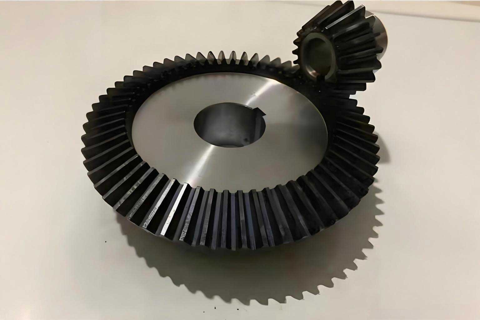
Although many advances have been made in the dynamic optimization of miter gear transmission systems, most studies treat the dynamic problem as a deterministic parameter problem. In engineering practice, uncertainties inevitably exist in manufacturing, machining, and assembly processes. If these uncertainties are not considered in the design optimization, the optimization results will deviate from reality, causing the dynamic performance of the miter gear transmission system to fluctuate over a large range and leading to premature failure. Strictly controlling manufacturing precision can eliminate some uncertainty, but it greatly increases production costs. Therefore, robust optimization research on the dynamics of high-speed miter gear transmission systems has important engineering significance.
In this article, I present my work on dynamic excitation characterization, dynamic modeling, vibration characteristic analysis, and robust optimization of high-speed miter gear transmission systems. I use first-person perspective to describe the methods, formulas, tables, and experimental validations. The miter gear system studied here is a single-stage high-speed miter gear transmission system. The basic parameters of the miter gear pair are listed in Table 1.
| Parameter | Value |
|---|---|
| High-speed gear teeth number z | 92 |
| Low-speed gear teeth number z | 46 |
| Module m | 7 mm |
| Normal pressure angle α | 25° |
| Tooth width b | 30 mm |
| Helix angle β | 23.38° |
| Density ρ | 7850 kg·m⁻³ |
| Elastic modulus E | 2.1×10¹¹ Pa |
| Poisson’s ratio | 0.3 |
| Undercut groove Bt | 10 |
| High-speed pitch line velocity | 169 m/s |
| Center distance | 530±0.0315 mm |
The dynamic excitation characterization of the high-speed miter gear transmission system is the foundation for accurate dynamic modeling. I first analyze the contact line length of the miter gear pair, then calculate the time-varying meshing stiffness using the energy method and verify it with the finite element method. I also characterize the transmission error, backlash, and bearing support stiffness and damping. These excitations directly affect the vibration response of the miter gear system.
The contact line length of a helical miter gear varies periodically during meshing. Depending on the relationship between the contact line motion velocity v₀ and the base pitch pbt, the contact line length L(t) can be expressed in three cases. When v₀ < pbt, the length is given by:
$$ L(t) = \begin{cases} v_0 t / \sin\beta_b, & t \in [t_0, t_1] \\ b / \cos\beta_b, & t \in [t_1, t_2] \\ (b \tan\beta_b + v_0 t – p_{bt}) / \sin\beta_b, & t \in [t_2, t_3] \\ 0, & t \in [t_3, T_n] \end{cases} $$
When v₀ = pbt, the contact line length becomes:
$$ L(t) = \begin{cases} v_0 t / \sin\beta_b, & t \in [t_0, t_1] \\ (b \tan\beta_b + v_0 t – p_{bt}) / \sin\beta_b, & t \in [t_1, t_2] \\ 0, & t \in [t_2, T_n] \end{cases} $$
When v₀ > pbt, the contact line length is:
$$ L(t) = \begin{cases} v_0 t / \sin\beta_b, & t \in [t_0, t_1] \\ p_{bt} / \sin\beta_b, & t \in [t_1, t_2] \\ (b \tan\beta_b + v_0 t – p_{bt}) / \sin\beta_b, & t \in [t_2, t_3] \\ 0, & t \in [t_3, T_n] \end{cases} $$
Here, v₀ = π d₁ n₁ / 60, where n₁ is the driving gear speed and d₁ is the base circle diameter. pbt is the transverse base pitch, and Tn is the meshing period of a single tooth. This periodic contact line length variation gives the miter gear pair a smooth transmission performance.
For time-varying meshing stiffness, I use the energy method. The potential energy stored in the meshing miter gear includes Hertzian energy Uh, bending energy Ub, compressive deformation energy Ua, and shear energy Us. The corresponding stiffness components are Kh, Kb, Ka, and Ks. The relationships are:
$$ U_h = \frac{F^2}{2K_h}, \quad U_b = \frac{F^2}{2K_b}, \quad U_a = \frac{F^2}{2K_a}, \quad U_s = \frac{F^2}{2K_s} $$
Under the meshing force F, the potential energies are:
$$ U_h = \frac{F^2}{2K_h}, \quad U_b = \int_0^d \frac{[F_b(d-x) – F_a h]^2}{2EI_x} dx, \quad U_s = \int_0^d \frac{1.2F_b^2}{2GA_x} dx, \quad U_a = \int_0^d \frac{F_a^2}{2EA_x} dx $$
The bending stiffness Kb is:
$$ \frac{1}{K_b} = \int_0^d \frac{[ (d-x)\cos\alpha_1 – h\sin\alpha_1 ]^2}{EI_x} dx $$
The shear stiffness Ks is:
$$ \frac{1}{K_s} = \int_0^d \frac{1.2\cos^2\alpha_1}{GA_x} dx $$
The axial compression stiffness Ka is:
$$ \frac{1}{K_a} = \int_0^d \frac{\sin^2\alpha_1}{EA_x} dx $$
The Hertzian contact stiffness Kh is:
$$ K_h = \frac{\pi E W}{4(1-\nu^2)} $$
The fillet foundation deformation stiffness Kf is calculated as:
$$ \delta_f = \frac{F}{W E} \left[ L^* \left( \frac{u_f}{S_f} \right)^2 + M^* \left( \frac{u_f}{S_f} \right) + P^* (1 + Q^* \tan^2\alpha_f) \right] $$
$$ \frac{1}{K_f} = \frac{\delta_f}{F} $$
For single tooth meshing, the total mesh stiffness is:
$$ K_e = \frac{1}{\frac{1}{K_h} + \frac{1}{K_{b1}} + \frac{1}{K_{s1}} + \frac{1}{K_{a1}} + \frac{1}{K_{f1}} + \frac{1}{K_{b2}} + \frac{1}{K_{s2}} + \frac{1}{K_{a2}} + \frac{1}{K_{f2}}} $$
For double tooth meshing, the stiffness is the sum of two pairs:
$$ K = \sum_{i=1}^{2} \frac{1}{\frac{1}{K_{h,i}} + \frac{1}{K_{b1,i}} + \frac{1}{K_{s1,i}} + \frac{1}{K_{a1,i}} + \frac{1}{K_{f1,i}} + \frac{1}{K_{b2,i}} + \frac{1}{K_{s2,i}} + \frac{1}{K_{a2,i}} + \frac{1}{K_{f2,i}}} $$
For helical miter gears, I use the slice theory. The gear is divided into multiple thin spur gear slices along the tooth width. Each slice has a thickness Δy. The bending potential energy of each slice is:
$$ dU_b = \frac{F^2}{2K_b} = \int_0^d \frac{[F_b(d-x) – F_a h]^2}{2EI_x} dy $$
After integration, the bending stiffness for the helical miter gear becomes:
$$ K_b = \int_0^b \frac{1}{\int_0^d \frac{[ (d-x)\cos\alpha_1 – h\sin\alpha_1 ]^2}{2EI_x} dy} db $$
The effective contact width beff is:
$$ b_{eff} = \begin{cases} b \cot\beta_b, & b < p_{bt} \\ b, & p_{bt} < b < p_{bt} + p_{et} \\ b – (b – p_{bt} – p_{et})\cot\beta_b, & p_{bt} + p_{et} < b \end{cases} $$
Similarly, the shear and axial compression stiffnesses are obtained by summation instead of integration. For n pairs of teeth in mesh, the total mesh stiffness is:
$$ K = \sum_{j=1}^{n} \frac{1}{\sum_{i=1}^{m} \left( \frac{1}{K_{h,i,j}} + \frac{1}{K_{b1,i,j}} + \frac{1}{K_{s1,i,j}} + \frac{1}{K_{a1,i,j}} + \frac{1}{K_{f1,i,j}} + \frac{1}{K_{b2,i,j}} + \frac{1}{K_{s2,i,j}} + \frac{1}{K_{a2,i,j}} + \frac{1}{K_{f2,i,j}} \right)} $$
I also use the finite element method to verify the time-varying meshing stiffness. The finite element model is built in a commercial software. The contact is set as frictional contact with a friction coefficient of 0.05. The mesh is tetrahedral with local refinement on the contact surfaces. The normal load and normal comprehensive elastic deformation are used to calculate the meshing stiffness. The comparison between the analytical method and finite element method is shown in Table 2. The results are very close, and the analytical method significantly improves calculation efficiency.
| Meshing position | Analytical stiffness (N/m) | Finite element stiffness (N/m) | Difference (%) |
|---|---|---|---|
| 1 | 2.68×10⁷ | 2.75×10⁷ | 2.6 |
| 2 | 2.74×10⁷ | 2.80×10⁷ | 2.1 |
| 3 | 2.81×10⁷ | 2.87×10⁷ | 2.1 |
| 4 | 2.76×10⁷ | 2.82×10⁷ | 2.1 |
| 5 | 2.70×10⁷ | 2.77×10⁷ | 2.5 |
| Average | 2.72×10⁷ | 2.80×10⁷ | 2.9 |
The transmission error of the miter gear pair is caused by elastic deformation, manufacturing error, assembly error, and thermal deformation. I use a harmonic function to simulate the actual transmission error. The expression is:
$$ e(t) = 0.5 E_p \sin(\omega_p t + \phi_p) + 0.5 E_g \sin(\omega_g t + \phi_g) $$
where Ep and Eg are the cumulative deviations, ωp and ωg are the rotational frequencies, and φp and φg are the initial phases. The comprehensive deviation is:
$$ E_g’ = 0.6 \times E_{pt} + E_{fa} $$
where Ept is the single pitch deviation and Efa is the profile deviation. The parameters for the high-speed and low-speed miter gears are listed in Table 3.
| Parameter | High-speed gear | Low-speed gear |
|---|---|---|
| Cumulative pitch deviation Ep (mm) | 0.034 | 0.044 |
| Pitch deviation Ept (mm) | 0.0085 | 0.0095 |
| Profile deviation Efa (mm) | 0.011 | 0.012 |
| Rotational frequency (r/s) | 100 | 50 |
| Meshing frequency (r/s) | 4600 | 4600 |
The backlash of the miter gear pair is necessary for assembly, lubrication, and heat dissipation. The backlash function is:
$$ b(t) = \begin{cases} \delta – b_0, & \delta > b_0 \\ 0, & |\delta| \le b_0 \\ \delta + b_0, & \delta < -b_0 \end{cases} $$
where b₀ is half of the normal average meshing backlash, and δ is the relative displacement along the meshing line without backlash. The minimum backlash is:
$$ 2b_{min} = \frac{2}{3} \times (0.06a + 0.0005d + 0.03m) $$
The maximum backlash is:
$$ 2b_{max} = E_{ss1} + E_{ss2} + 2f_a \tan\alpha \cos\beta + \Delta_a $$
For the bearing support, I use sliding bearings. The bearing support is simplified as massless springs and dampers. I use DyRoBeS software to calculate the bearing stiffness and damping. The results are shown in Table 4.
| Bearing | High-speed bearing 1-2 | Low-speed bearing 3-4 |
|---|---|---|
| Stiffness (N/mm) | kxx=5.859×10⁵, kxy=1.194×10⁵, kyx=-1.093×10⁵, kyy=8.763×10⁵ | kxx=6.968×10⁵, kxy=-1.480×10⁵, kyx=-8.701×10⁵, kyy=5.709×10⁵ |
| Damping (N·s/mm) | cxx=1.015×10³, cxy=-7.841×10², cyx=-7.841×10², cyy=3.259×10³ | cxx=1.849×10³, cxy=-1.714×10², cyx=-1.714×10², cyy=3.241×10³ |
Based on the flexible multibody dynamics theory, I establish the dynamic simulation model of the high-speed miter gear transmission system. The motion of a flexible body is divided into rigid body motion and flexible deformation. The generalized coordinates are:
$$ \xi = [x, y, z, \psi, \theta, \phi, q]^T = [r, \psi, q]^T $$
The position vector of any point after rigid body motion and flexible deformation is:
$$ r_p = r + A(s_p + \Phi_p q) $$
The first derivative gives the velocity vector:
$$ \dot{r}_p = \dot{r} + A \dot{s}_p + A \Phi_p \dot{q} = [E – A \tilde{s}_p B + A \Phi_p] \dot{\xi} $$
The flexible body dynamic equation is:
$$ M \ddot{\xi} + M \dot{\xi} – \frac{1}{2} \left( \frac{\partial M}{\partial \xi} \dot{\xi} \right)^T \dot{\xi} + K \xi + D \dot{\xi} + \left( \frac{\partial \Psi}{\partial \xi} \right)^T \lambda = Q $$
where M, K, and D are the mass, stiffness, and damping matrices, respectively. Ψ is the constraint equation, λ is the Lagrange multiplier, and Q is the generalized force.
I perform modal analysis of the high-speed miter gear transmission system. The first eight natural frequencies and main mode shapes are listed in Table 5. The first natural frequency is 131.16 Hz, and the second is 164.98 Hz. The working rotational frequency of the high-speed shaft is 100 Hz, which is far less than the first natural frequency. The meshing frequency is 4600 Hz, which is much larger than the first eight natural frequencies. Therefore, the gearbox will not resonate in the working speed range.
| Order | Natural frequency (Hz) | Main mode shape |
|---|---|---|
| 1 | 131.16 | Torsion of gear shaft and swing of box along Y axis |
| 2 | 164.98 | First bending of low-speed gear shaft and swing of box along X axis |
| 3 | 202.49 | Expansion of box along Z axis |
| 4 | 209.09 | First bending of low-speed gear shaft and torsion of box around Z axis |
| 5 | 238.18 | First bending of low-speed gear shaft and expansion of box bottom around Z axis |
| 6 | 282.47 | Expansion of box bottom along Z axis |
| 7 | 307.48 | Torsion of box and bending deformation of low-speed shaft |
| 8 | 316.59 | Expansion of box bottom around Z axis |
I also analyze the critical speed of the miter gear rotor system. The critical speed is the speed at which the rotor natural frequency coincides with the excitation frequency. The Campbell diagram is used. The first two critical speeds are 14908 r/min and 36286 r/min. The rated speed of the miter gear transmission system is 6000 r/min, which is much lower than the first critical speed. Therefore, the miter gear shaft system operates stably in the normal working speed range. The critical speed results are listed in Table 6.
| Mode | Rotation direction | Mode stability | Critical speed (r/min) |
|---|---|---|---|
| 1 | BW | Stable | 13062 |
| 2 | FW | Stable | 14908 |
| 3 | BW | Stable | 29598 |
| 4 | BW | Stable | 30057 |
| 5 | BW | Stable | 36286 |
To identify potential resonance points of the high-speed miter gear transmission system, I propose three principles: the frequency principle, the damping principle, and the energy principle. The frequency principle sets the upper limit of the excitation frequency to six times the rotational frequency of the high-speed shaft or three times the meshing frequency. The damping principle ignores undamped, critically damped, and overdamped modes, retaining only modes with damping ratio 0 < ζ < 1. The energy principle states that if the sum of rotational energies of all components in the miter gear system at a certain natural frequency is less than 1, the system will not be excited to resonate at that frequency. The energy expression is:
$$ E_1 + E_2 + E_3 + \cdots + E_n < 1 $$
After screening, the 8th natural frequency at 164.98 Hz is retained as a potential resonance point. Since the working speed is 6000 r/min, the miter gear system will not resonate at this frequency. The energy distribution and screening results are shown in Table 7.
| Order | Frequency (Hz) | Total energy (kin./modal) |
|---|---|---|
| 8 | 164.98 | 2.2911 |
I analyze the vibration characteristics of the high-speed miter gear transmission system using the modal superposition method. The time step is 0.01 s, and the total solution time is 0.1 s. Four evaluation points are selected. Points 1 and 2 are at the input and output shaft centers, respectively. Points 3 and 4 are on the top of the gearbox above the high-speed and low-speed gear shafts. The vibration displacements at different speeds are listed in Table 8. The results show that the input shaft vibration is larger than the output shaft vibration, and the vibration increases with increasing speed.
| Speed (r/min) | Point | Direction | Displacement (μm) |
|---|---|---|---|
| 3000 | 1 | X | 14.86 |
| 1 | Y | 13.97 | |
| 2 | X | 6.1 | |
| 2 | Y | 5.5 | |
| 4000 | 1 | X | 17.46 |
| 1 | Y | 15.57 | |
| 2 | X | 7.48 | |
| 2 | Y | 6.68 | |
| 5000 | 1 | X | 18.95 |
| 1 | Y | 18.71 | |
| 2 | X | 12.11 | |
| 2 | Y | 10.34 | |
| 6000 | 1 | X | 22.87 |
| 1 | Y | 20.27 | |
| 2 | X | 15.32 | |
| 2 | Y | 13.63 |
The vibration acceleration of the gearbox at 6000 r/min is also analyzed. The root mean square values of acceleration at points 3 and 4 are listed in Table 9. The results show that the vibration acceleration in the X and Y directions is larger than in the Z direction. The overall vibration acceleration is relatively small, indicating stable operation of the miter gear system.
| Evaluation point | Direction | Acceleration (mm/s²) |
|---|---|---|
| 3 | X | 5881.5 |
| Y | 4408.2 | |
| Z | 4285.9 | |
| 4 | X | 5778.4 |
| Y | 5439.7 | |
| Z | 3923.1 |
For robust optimization design, I consider uncertainties in manufacturing, assembly, and operation. The robust optimization design aims to reduce the sensitivity of the miter gear dynamic response to parameter uncertainties. The basic elements include signal factors, noise factors, design variables, and quality characteristics. The two objectives are to minimize variance and minimize deviation:
$$ \sigma_y^2 = E(y – \bar{y})^2 \rightarrow \min $$
$$ \delta_y^2 = E(\bar{y} – y_0)^2 \rightarrow \min $$
I establish a 6σ robust optimization design model for the high-speed miter gear transmission system. The objective is to minimize the vibration acceleration of the gearbox. The design variables are seven thickness parameters: gear cover thickness x₁, gearbox thickness x₂, bottom plate thickness x₃, reinforcement plate thickness x₄, small block thickness x₅, inner support plate thickness x₆, and crossbeam thickness x₇. The initial values and ranges are listed in Table 10.
| Variable | Meaning | Initial value (mm) | Range (mm) | Distribution |
|---|---|---|---|---|
| x₁ | Gear cover thickness | 14 | 9~19 | Normal |
| x₂ | Gearbox thickness | 24 | 19~29 | Normal |
| x₃ | Bottom plate thickness | 14 | 9~19 | Normal |
| x₄ | Reinforcement plate thickness | 10 | 5~15 | Normal |
| x₅ | Small block thickness | 24 | 19~29 | Normal |
| x₆ | Inner support plate thickness | 24 | 19~29 | Normal |
| x₇ | Crossbeam thickness | 90 | 80~100 | Normal |
The objective function is:
$$ f_1(x) = \frac{1}{n} \sum_{i=1}^{n} a_i $$
where ai is the root mean square value of vibration acceleration at evaluation point i, and n = 2. The 6σ robust optimization model is:
$$ \text{Minimize } F(\mu_f(x), \sigma_f(x)) $$
$$ \text{Subject to } G_j(\mu_g(x), \sigma_g(x)) \le 0 $$
$$ x_{L} + \Delta x \le x \le x_{U} – \Delta x $$
The objective function F can be decomposed into mean and variance:
$$ F = \sum_{i=1}^{l} \left[ \frac{w_1}{\sigma_1} (\mu_f – M)^2 + \frac{w_2}{\sigma_2} \sigma_f^2 \right] $$
where w₁ and w₂ are weight coefficients, σ₁ and σ₂ are proportional coefficients, M is the target mean, and l is the number of objectives.
I use Latin hypercube sampling to generate 20 sample points. The sensitivity analysis shows that the reinforcement plate thickness and bottom plate thickness have the most significant influence on the vibration acceleration of the miter gearbox. The fitting curve shows good agreement between the predicted and actual values. The sensitivity histogram is shown in Table 11.
| Design variable | Sensitivity (%) |
|---|---|
| x₁ (cover) | 8.2 |
| x₂ (gearbox) | 7.5 |
| x₃ (bottom plate) | 18.6 |
| x₄ (reinforcement plate) | 21.3 |
| x₅ (small block) | 9.1 |
| x₆ (inner support plate) | 10.4 |
| x₇ (crossbeam) | 6.8 |
I use the Kriging interpolation method to construct the response surface. The response surface analysis shows that the seven design variables affect the directional acceleration. However, in specific regions, the variation of design variables does not cause sharp changes in directional acceleration. Therefore, optimization can reduce the sensitivity of vibration acceleration to design variable uncertainties. The optimized design variable values are listed in Table 12. The gearbox mass is reduced by 58.712 kg.
| Variable | Initial value (mm) | Optimal value (mm) | Rounded value (mm) |
|---|---|---|---|
| x₁ | 14 | 12.4857 | 12 |
| x₂ | 24 | 22.1458 | 22 |
| x₃ | 14 | 15.4265 | 15 |
| x₄ | 10 | 11.3906 | 11 |
| x₅ | 24 | 27.3374 | 27 |
| x₆ | 24 | 20.2262 | 20 |
| x₇ | 90 | 80.2657 | 80 |
The comparison of vibration acceleration before and after optimization is shown in Table 13. The acceleration at points 3 and 4 in all three directions is significantly reduced. The reduction ratios are 45.2%, 33.7%, 30.4%, 42.6%, 41.1%, and 26.1%, respectively. The probability density distributions of the design variables before and after optimization are analyzed. The standard deviations change only slightly, indicating improved robustness. The reliability and σ levels are shown in Table 14. The reliability of the bottom plate thickness at 15.4265 mm is 98.6%, the reinforcement plate thickness at 11.3903 mm is 99.7%, and the cover thickness at 12.4857 mm is 97.2%. These results verify the effectiveness and reliability of the robust optimization method.
| Evaluation point | Direction | Before optimization (mm/s²) | After optimization (mm/s²) | Reduction (%) |
|---|---|---|---|---|
| 3 | X | 5881.5 | 3224.2 | 45.2 |
| Y | 4408.2 | 2908.3 | 33.7 | |
| Z | 4285.9 | 2901.5 | 30.4 | |
| 4 | X | 5778.4 | 3312.7 | 42.6 |
| Y | 5439.7 | 3205.4 | 41.1 | |
| Z | 3923.1 | 2899.6 | 26.1 |
| Parameter | Optimal value (mm) | Reliability | σ level |
|---|---|---|---|
| Bottom plate thickness | 15.4265 | 98.6% | 2.21 |
| Reinforcement plate thickness | 11.3903 | 99.7% | 2.80 |
| Cover thickness | 12.4857 | 97.2% | 1.91 |
To validate the optimized high-speed miter gear transmission system, I manufactured a prototype of the optimized miter gearbox. I built a comprehensive performance test bench. The test bench mainly measures shaft vibration displacement, gearbox vibration acceleration, temperature rise, power consumption, and noise. The layout includes a motor, sensors, a speed-increasing gearbox, and the tested miter gearbox. Eddy current sensors are installed at the input and output bearings to collect shaft vibration signals. The probe distance from the shaft is 1 mm, and the probes are placed at 45 degrees to the horizontal and vertical directions, defining X and Y channels. Four triaxial acceleration sensors are placed on the top of the gearbox, each directly above the gear axis and 20 cm from the side of the gearbox. The instruments include eddy current sensors, triaxial acceleration sensors, NI9231 and NI9215 acquisition cards, a cDAQ chassis, a Fluke tix 580 infrared thermometer, and a noise meter. The parameters are listed in Table 15.
| Instrument | Model | Key parameters |
|---|---|---|
| Eddy current sensor | 3300 XL 8MM | Gap voltage -11 V, max range 2 mm |
| Triaxial acceleration sensor | 3273A2 | Sensitivity 103 mV/g, range ±500 m/s² |
| NI-9231 | 8 channels | 24-bit, 51200 S/s, synchronous |
| NI-9215 | 4 channels | 24-bit, 51200 S/s, synchronous |
| cDAQ chassis | 8 slots | 50 ppm, 12.5 ns |
| Infrared thermometer | Fluke tix 580 | -20°C to +1000°C, ≤0.05°C |
The experimental procedure is as follows. First, the lubrication system pressure is set to 130000 Pa. After the lubrication is stable, the input speed is adjusted to 500 r/min, 1000 r/min, 2000 r/min, and 3000 r/min, and the miter gearbox is checked for abnormal operation. Then the input speed is set to 6000 r/min, and the tested gearbox runs continuously for 1 hour. The bearing temperature rise is checked. Then the speed is increased to 6600 r/min for 20 minutes. After confirming stable operation, the machine is stopped, and all connections and fasteners are checked. Second, the acquisition card is connected to the computer, the sampling rate is set to 15000 Hz, and the speed is slowly increased from 3000 r/min to 6000 r/min in steps of 200 r/min, with 2 minutes at each step. When the shaft vibration displacement reaches a stable state, the data are recorded for 30 seconds. At the same time, at speeds of 500 r/min, 1200 r/min, 3000 r/min, and 5400 r/min, the oil inlet and outlet temperatures, bearing temperature, and oil inlet pressure are recorded. Third, at 6000 r/min, after stable operation, the oil inlet and outlet temperatures, bearing temperature, and oil inlet pressure are recorded. Fourth, at 6000 r/min, the miter gearbox runs stably for 2 hours, and the data are recorded every 5 minutes.
The shaft vibration displacement at 6000 r/min is analyzed. The time-domain diagrams for points 1 and 2 are obtained. The vibration displacement values at different speeds are listed in Table 16. The results show that the miter gearbox shaft vibration is small and stable. The vibration displacement increases with speed. At the same speed, the vibration response at point 1 is generally larger than at point 2 because the input shaft bears the largest load. At the rated speed of 6000 r/min, the maximum radial shaft vibration is 19.1 μm.
| Speed (r/min) | Point 1 X (μm) | Point 1 Y (μm) | Point 2 X (μm) | Point 2 Y (μm) |
|---|---|---|---|---|
| 3000 | 12.56 | 11.57 | 4.77 | 4.49 |
| 4000 | 13.73 | 13.56 | 5.04 | 4.54 |
| 5000 | 16.43 | 15.73 | 8.51 | 8.19 |
| 6000 | 19.1 | 17.5 | 9.46 | 8.67 |
The gearbox vibration acceleration at 6000 r/min is also measured. The root mean square values of acceleration at points 3 and 4 are listed in Table 17. The results show that the vibration acceleration in the X and Y directions is similar, while the Z direction is slightly smaller. The overall vibration acceleration is small, indicating that the miter gearbox operates stably at the rated speed and meets the design requirements.
| Evaluation point | X direction (m/s²) | Y direction (m/s²) | Z direction (m/s²) |
|---|---|---|---|
| 3 | 3.187 | 2.811 | 2.098 |
| 4 | 2.776 | 2.491 | 1.807 |
The temperature rise experiment is conducted at 6000 r/min. The bearing temperatures are stable. The measured data are listed in Table 18. The power consumption experiment is conducted at input speeds from 500 to 6000 r/min. The measured data are listed in Table 19. The power consumption ratio at 6000 r/min is 1.14%. The noise experiment is conducted at 6000 r/min. The noise is measured at 1 meter from the miter gearbox at three test points. The measured values are listed in Table 20. All indicators meet the design requirements.
| Measurement | Low-speed shaft input | Low-speed shaft output | High-speed shaft input | High-speed shaft output | Oil inlet | Oil outlet | Room temperature |
|---|---|---|---|---|---|---|---|
| Temperature (°C) | 54.8 | 56.8 | 53.4 | 48.5 | 46.5 | 58.3 | 29 |
| Input speed (r/min) | Input torque (Nm) | Power consumption (kW) | Power consumption ratio (%) |
|---|---|---|---|
| 500 | 44 | 2.3 | 0.01 |
| 1200 | 89 | 11.2 | 0.06 |
| 3000 | 222 | 69.6 | 0.35 |
| 5400 | 338 | 191.5 | 0.96 |
| 6000 | 362 | 227.2 | 1.14 |
| Test point | Measured value (dB(A)) |
|---|---|
| 1 | 111.7 |
| 2 | 106.5 |
| 3 | 109.5 |
In conclusion, I have studied the dynamic excitation characterization, dynamic modeling, vibration characteristic analysis, and robust optimization of high-speed miter gear transmission systems. The main conclusions are as follows. First, I established a time-varying meshing stiffness model of the miter gear based on the energy method and verified it with the finite element method. I introduced the static transmission error using harmonic superposition of rotational and meshing frequencies. I analyzed the backlash and solved the minimum and maximum clearances. I calculated the sliding bearing support stiffness and damping using DyRoBeS software. Second, I established a dynamic finite element simulation model of the high-speed miter gear transmission system. I analyzed the gearbox modal and rotor critical speeds. I proposed three resonance point screening principles: frequency principle, damping principle, and energy principle. I analyzed the shaft vibration response and gearbox surface acceleration at different speeds. Third, I established a 6σ robust optimization design model for the dynamic performance of the high-speed miter gear transmission system. The objective was to reduce the vibration acceleration response of the gearbox. Through sensitivity analysis, I obtained the influence of different gearbox dimension design variables on the vibration response. I used the Kriging interpolation method for response surface analysis. The vibration acceleration at points 3 and 4 in three directions decreased by 45.2%, 33.7%, 30.4%, 42.6%, 41.1%, and 26.1%, respectively. The probability density distributions and reliability of the design variables before and after optimization verified the effectiveness of the robust optimization design method. Fourth, based on the optimized gearbox parameters, I manufactured a prototype of the optimized high-speed miter gearbox. I conducted experiments on shaft vibration displacement, gearbox vibration acceleration, temperature rise, power consumption, and noise. The performance of the prototype meets the design requirements. Future work should consider more uncertainties such as tooth friction, thermal deformation, and interface stiffness to further improve the accuracy of dynamic modeling and robust optimization of high-speed miter gear transmission systems.