
In modern industrial robotics, high-precision reducers play a pivotal role in ensuring accurate motion control and operational efficiency. Among these, the rotary vector reducer, commonly known as the RV reducer, is extensively utilized in robot joints due to its compact design, high torque capacity, and excellent backlash performance. However, during prolonged operation, wear of critical components such as the cycloidal gear can degrade transmission accuracy, leading to increased backlash and reduced robotic precision. This paper addresses this issue by developing a dynamic reliability model for the transmission accuracy of rotary vector reducers, incorporating cycloidal gear wear, and conducting a comprehensive parameter optimization to enhance performance and longevity. We focus on a heavy-duty rotary vector reducer as a case study, employing numerical simulations and multi-objective optimization techniques to provide insights for designing high-precision reducers.
The transmission accuracy of a rotary vector reducer is influenced by both static factors, such as manufacturing tolerances and assembly errors, and dynamic factors, including time-varying stiffness, elastic deformations, and wear. While previous studies have explored static error contributions, the impact of progressive wear on dynamic accuracy remains underexplored. In this work, we establish a framework that integrates wear prediction into reliability analysis, enabling a holistic assessment of reducer performance over its operational life. Our approach leverages the Archard wear model to quantify cycloidal gear wear, Gaussian process regression for efficient wear prediction, and Monte Carlo simulations for reliability evaluation. By optimizing key parameters, we aim to minimize manufacturing costs and wear while maintaining high transmission accuracy reliability.
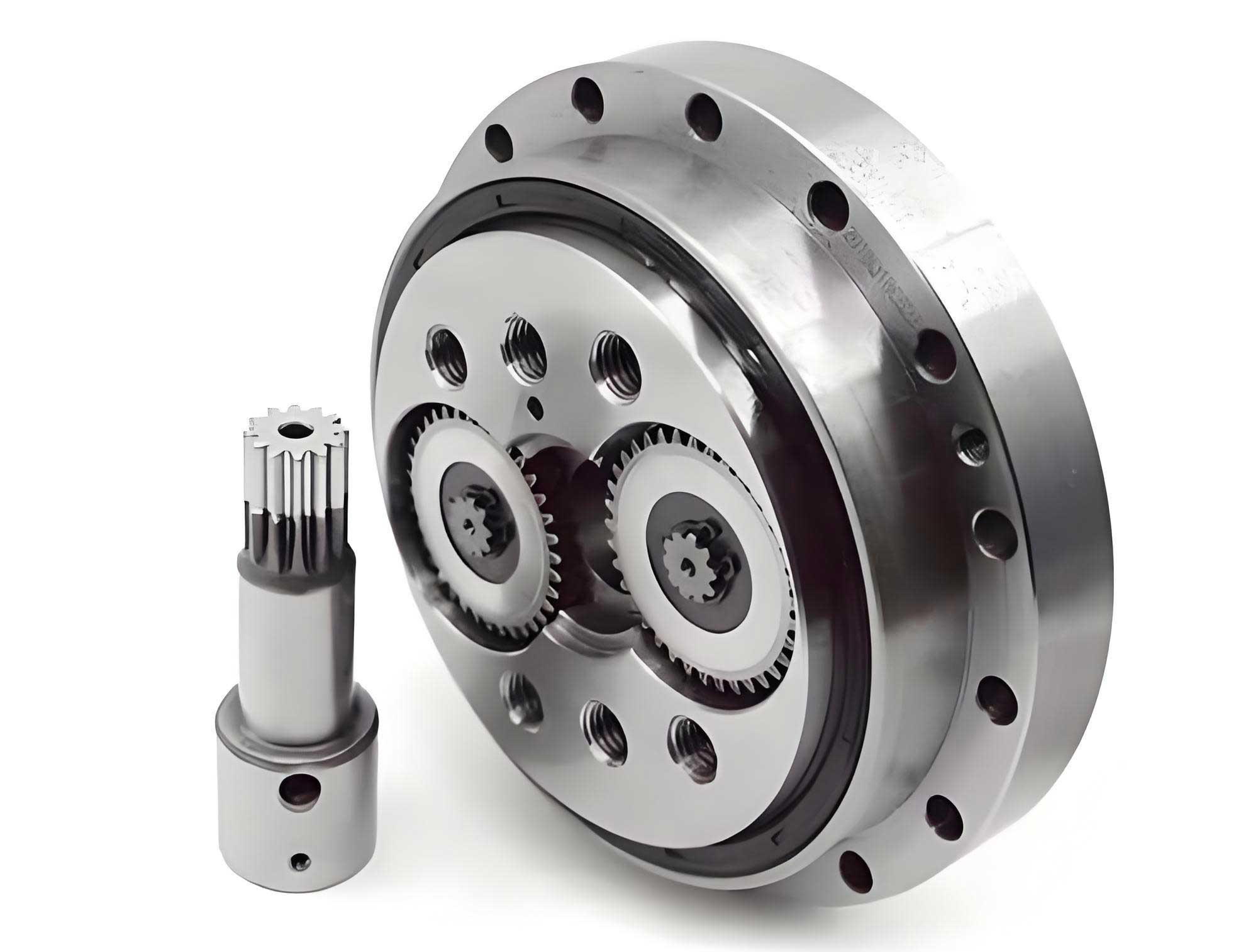
The structure of a rotary vector reducer typically consists of a two-stage reduction mechanism: a first-stage involute planetary gear train and a second-stage cycloidal-pin gear transmission. The cycloidal gear, driven by an eccentric crankshaft, engages with multiple pins to achieve high reduction ratios and low backlash. However, the multi-tooth contact and sliding motions in the cycloidal drive induce wear, which gradually alters the gear profile and increases clearance. This wear process is stochastic and time-dependent, necessitating a dynamic reliability approach. In the following sections, we detail our methodology for wear calculation, reliability modeling, and optimization, presenting results that demonstrate the effectiveness of our proposed framework for improving rotary vector reducer design.
Numerical Calculation and Prediction of Cycloidal Gear Wear
Wear in cycloidal gears arises from repeated sliding contact with pins under load. To quantify this wear, we adopt the Archard wear model, which relates wear volume to sliding distance, load, and material properties. For a rotary vector reducer, the wear depth at each meshing point on the cycloidal gear tooth profile can be computed by integrating contact pressures, sliding distances, and wear coefficients over time. This section outlines the step-by-step procedure for wear calculation and prediction, incorporating numerical simulations and regression modeling.
Calculation of Contact Pressure in Cycloidal-Pin Engagement
The cycloidal-pin transmission involves multiple simultaneous contacts, making force distribution complex. We use a numerical approach to determine the meshing forces. Initially, the maximum meshing force \( F_{\text{max}} \) is estimated based on the transmitted torque and geometry. The Hertz contact theory is applied to compute the deformation at the point of maximum force. Considering profile modifications that introduce initial backlash, we assume a linear relationship between the meshing force \( F_i \) and the difference between deformation and initial clearance for each theoretical meshing point \( i \). The equations are as follows:
The initial maximum force \( F_{\text{max0}} \) is given by:
$$ F_{\text{max0}} = \frac{4 T_c}{K_1 z_c r_p} $$
where \( T_c \) is the torque transmitted by the cycloidal gear, \( K_1 \) is the short-width coefficient, \( z_c \) is the number of cycloidal gear teeth, and \( r_p \) is the pitch circle radius of the pins. The deformation \( \delta_{\text{max}} \) at the maximum force point is derived from Hertz contact formulas.
The meshing force at point \( i \) with phase angle \( \psi_i \) is expressed as:
$$ F_i = \frac{F_{\text{max}}}{\delta_{\text{max}}} (\delta_i – \Delta s_i) $$
where \( \delta_i \) is the total normal displacement at the theoretical meshing point, and \( \Delta s_i \) is the initial clearance at that point. Points where \( \delta_i > \Delta s_i \) are considered to be in contact, allowing us to identify the meshing region and the number of simultaneously engaged teeth. The torque balance equation for the cycloidal gear is:
$$ T_c = \sum_{i=M}^{N} F_i l_i $$
with \( l_i \) being the distance from the contact normal to the cycloidal gear center. By rearranging, we obtain an iterative formula for \( F_{\text{max}} \):
$$ F_{\text{max}} = \frac{T_c}{\sum_{i=M}^{N} \left( \frac{l_i}{l_{\text{max}}} – \frac{\Delta s_i}{\delta_{\text{max}}} \right) l_i} $$
where \( l_{\text{max}} \) is the pitch radius of the cycloidal gear. Iteration continues until \( F_{\text{max0}} \) and \( F_{\text{max}} \) converge, yielding final meshing forces.
The average contact pressure \( p_i \) on the cycloidal gear tooth surface at point \( i \) is then:
$$ p_i = \frac{F_i}{2b B} $$
where \( b \) is the half-width of contact, and \( B \) is the tooth width of the cycloidal gear.
Determination of Sliding Distance
Relative sliding between the cycloidal gear and pins contributes to wear. The relative sliding velocity \( v_r \) is computed from kinematic analysis:
$$ v_r = – \left( r_p \sqrt{s} – \frac{1}{2} – r_{rp} \right) \frac{\omega_H}{z_c} $$
with \( s = 1 + K_1^2 – 2K_1 \cos \psi_i \), \( r_{rp} \) as the pin radius, and \( \omega_H \) as the angular velocity of the crankshaft. The sliding coefficient \( \lambda \), defined as the ratio of sliding velocity to tangential velocity, is:
$$ \lambda = \frac{v_r}{v_t} $$
The sliding distance per engagement \( du \) for a contact point is:
$$ du = 2b \lambda $$
Estimation of Wear Coefficient
The wear coefficient \( k \) is a dynamic parameter influenced by operational conditions and material properties. Based on experimental regressions by Janakiraman et al., we estimate \( k \) using dimensionless parameters:
$$ k = \frac{3.981 \times 10^{29}}{E’} L^{1.219} G^{-7.377} S^{1.589} $$
where \( E’ \) is the equivalent elastic modulus, and \( L \), \( G \), and \( S \) are dimensionless load, pressure-viscosity coefficient, and composite surface roughness, respectively, defined as:
$$ L = \frac{W’}{E’ R’}, \quad G = \alpha E’, \quad S = \frac{R_{cq}}{\sqrt{R’}} $$
Here, \( W’ \) is the unit line load, \( R’ \) is the equivalent curvature radius, \( \alpha \) is the pressure-viscosity coefficient, and \( R_{cq} \) is the composite surface roughness. This formulation captures the influence of lubrication and surface conditions on wear, which is critical for rotary vector reducers operating under varying loads.
Computation of Wear Depth
Using the Archard model, the wear depth per engagement \( dh \) at a point is:
$$ dh = k p_i du $$
The meshing period \( t \), i.e., the time for all teeth to engage once, is:
$$ t = \frac{2\pi}{z_p – 1} \frac{z_p}{\omega_H} $$
where \( z_p \) is the number of pins. As wear accumulates, the tooth profile changes, altering contact pressures. We divide the wear process into intervals with a threshold \( \varepsilon \), within which wear per engagement is assumed constant. The cumulative wear depth \( h_q \) over a reconstruction period \( t_q \) is:
$$ h_q = \frac{1}{t} t_q dh $$
The total wear depth over operational time \( T \) is:
$$ h = \sum_{q=1}^{Q} h_q $$
where \( Q \) is the number of reconstruction intervals.
Profile modifications, such as equidistant and shift modifications, affect the meshing pattern and forces, thereby influencing wear distribution. For a specific heavy-duty rotary vector reducer, we analyze wear under different modification combinations. The parameters of the reducer are listed in Table 1.
| Parameter | Value | Parameter | Value |
|---|---|---|---|
| Number of cycloidal gear teeth, \( z_c \) | 39 | Shift modification amount, \( \Delta r_p \) (mm) | -0.030 |
| Number of pins, \( z_p \) | 40 | Elastic modulus (GPa) | 206 |
| Pin radius, \( r_{rp} \) (mm) | 5 | Poisson’s ratio | 0.3 |
| Pin pitch circle radius, \( r_p \) (mm) | 114.5 | Sun gear pitch radius (mm) | 15 |
| Eccentricity, \( e \) (mm) | 2.2 | Center distance (mm) | 63 |
| Cycloidal gear tooth width, \( B \) (mm) | 18 | Involute gear pressure angle (°) | 20 |
| Equidistant modification amount, \( \Delta r_{rp} \) (mm) | -0.026 | Rated load, \( T_z \) (N·m) | 3136 |
By varying equidistant modification within the range \([-0.053, 0.011]\) mm and adjusting shift modification to maintain initial radial clearance, we compute meshing forces and wear after 100 hours of operation. Results indicate that larger equidistant modification reduces maximum meshing force, expands the contact region, and leads to more uniform wear distribution across the tooth profile. This highlights the importance of modification parameters in managing wear for rotary vector reducers.
Wear Prediction Using Gaussian Process Regression
Given the computational expense of repeated wear simulations, we employ Gaussian process regression (GPR) to predict wear based on limited simulation data. GPR is a non-parametric Bayesian approach suitable for small datasets and uncertainty quantification. We train the model with inputs including load \( T_z \), speed \( n \), operating time \( T \), and modification amounts, and output the corresponding wear depth. The joint Gaussian distribution of observed wear \( w_o \) and predicted wear \( w_p \) is:
$$ \begin{bmatrix} w_o \\ w_p \end{bmatrix} \sim \mathcal{N} \left( 0, \begin{bmatrix} K_{oo} + \sigma^2 I & K_{op} \\ K_{po} & K_{pp} \end{bmatrix} \right) $$
where \( K_{oo} \), \( K_{op} \), \( K_{po} \), and \( K_{pp} \) are covariance matrices, and \( \sigma^2 \) is noise variance. The predictive distribution is:
$$ w_p \sim \mathcal{N} \left( K_{po}[K_{oo} + \sigma^2 I]^{-1} w_o, K_{pp} – K_{po}[K_{oo} + \sigma^2 I]^{-1} K_{op} \right) $$
We validate the model by comparing simulated and predicted wear for a scenario with \( T_z = 3136 \, \text{N·m} \), \( n = 15 \, \text{r/min} \), \( T = 3000 \, \text{h} \), \( \Delta r_{rp} = -0.026 \, \text{mm} \), and \( \Delta r_p = -0.030 \, \text{mm} \). Predictions fall within the 95% confidence interval, demonstrating accuracy. This GPR model enables efficient wear forecasting for reliability analysis without extensive simulations.
Dynamic Reliability Analysis of Transmission Accuracy Incorporating Wear
Transmission accuracy in rotary vector reducers is commonly assessed via backlash, which stems from clearances due to manufacturing tolerances, assembly errors, and wear. We develop a dynamic reliability model that accounts for time-dependent wear of the cycloidal gear, alongside static error sources. The model evaluates the probability that backlash remains within allowable limits over the reducer’s operational life, providing a robust measure of performance degradation.
Modeling Backlash with Wear Inclusion
Total backlash \( \Delta \phi \) in a rotary vector reducer is the angular displacement lost due to clearances. It is expressed as a function of normal clearances \( \Delta \beta_j \) induced by various error factors, including wear. Based on prior studies, we list these error factors and their contributions in Table 2.
| Index \( j \) | Error Factor | Normal Backlash \( \Delta \beta_j \) | Sensitivity Index \( s_j \) |
|---|---|---|---|
| 1 | Base tangent length deviation, \( E_w \) | \( -\frac{E_w}{\cos \theta} \) | -0.037 |
| 2 | Gear radial runout error, \( \Delta f_r \) | \( 2 \Delta f_r \tan \theta \) | 0.025 |
| 3 | Center distance error, \( \Delta f_a \) | \( 2 \Delta f_a \tan \theta \) | 0.025 |
| 4 | Equidistant modification amount, \( \Delta r_{rp} \) | \( 2 \Delta r_{rp} \) | 1.56 |
| 5 | Shift modification amount, \( \Delta r_p \) | \( -2 \Delta r_p \sqrt{1 – K_1^2} \) | -1 |
| 6 | Pin pitch circle radius error, \( \delta r_p \) | \( 2 \delta r_p \sqrt{1 – K_1^2} \) | 1 |
| 7 | Pin radius error, \( \delta r_{rp} \) | \( -2 \delta r_{rp} \) | -1.56 |
| 8 | Pin-sleeve fit clearance, \( \delta J \) | \( \frac{\delta J}{2} \) | 0.78 |
| 9 | Cycloidal gear radial runout error, \( \Delta F_r \) | \( \frac{\Delta F_r}{2} \) | 0.39 |
| 10 | Pin hole circumferential position error, \( \delta t \) | \( K_1 \delta t \) | 1.20 |
| 11 | Cycloidal gear profile cumulative error, \( F_{pk} \) | \( -\frac{K_1 F_{pk}}{2} \) | -0.60 |
| 12 | Equidistant modification error, \( \delta \Delta r_{rp} \) | \( 2 \delta \Delta r_{rp} \) | 1.56 |
| 13 | Shift modification error, \( \delta \Delta r_p \) | \( -2 \delta \Delta r_p \sqrt{1 – K_1^2} \) | -1 |
| 14 | Eccentricity error, \( \delta a \) | \( 2 k_n \delta a \) | 0.00016 |
| 15 | Cycloidal gear profile wear, \( \delta w \) | \( 2 \delta w \) | 1.56 |
| 16 | Crankshaft bearing clearance, \( \Delta r \) | \( \Delta r \) | 1.06 |
Note: \( \theta \) is the pressure angle of involute gears, and \( k_n \) is an error factor. The sensitivity index \( s_j \) is relative to the pin pitch circle radius error, indicating each factor’s influence on total backlash.
The total backlash \( \Delta \phi \) in arc-minutes is computed as:
$$ \Delta \phi = \frac{180 \times 60}{\pi} \left( \sum_{j=1}^{3} \frac{\Delta \beta_j}{i_H r_1} + \sum_{j=4}^{15} \frac{\Delta \beta_j}{e z_c} + \frac{\Delta \beta_{16}}{a} \right) $$
where \( i_H \) is the reduction ratio, \( r_1 \) is the sun gear pitch radius, and \( a \) is the center distance between sun and planetary gears. Wear depth \( \delta w \) from the cycloidal gear contributes directly to \( \Delta \beta_{15} \), making backlash time-dependent as wear accumulates.
Dynamic Reliability Assessment
We define the reliability function \( g(\mathbf{x}, \Delta \phi_{\text{per}}) \) as:
$$ g(\mathbf{x}, \Delta \phi_{\text{per}}) = \Delta \phi – \Delta \phi_{\text{per}} $$
where \( \mathbf{x} = (T_z, n, T, \Delta r_{rp}, \Delta r_p) \) is the vector of operational and design parameters, and \( \Delta \phi_{\text{per}} \) is the permissible backlash. Failure occurs when \( g > 0 \), meaning backlash exceeds the allowable limit. Since manufacturing errors and wear are random, we treat them as random variables with known distributions, as summarized in Table 3.
| Parameter | Deviation Value (mm) | Distribution |
|---|---|---|
| Base tangent length deviation, \( E_w \) | -0.049 | Normal |
| Gear radial runout error, \( \Delta f_r \) | -0.086 | Rayleigh |
| Center distance error, \( \Delta f_a \) | 0.014 | Normal |
| Pin pitch circle radius error, \( \delta r_p \) | ±0.01 | Normal |
| Pin radius error, \( \delta r_{rp} \) | ±0.0025 | Normal |
| Pin-sleeve fit clearance, \( \delta J \) | -0.0075 to +0.010 | Normal |
| Cycloidal gear radial runout error, \( \Delta F_r \) | -0.0087 to +0.005 | Rayleigh |
| Pin hole circumferential position error, \( \delta t \) | ±0.005 | Normal |
| Cycloidal gear profile cumulative error, \( F_{pk} \) | 0.015 | Normal |
| Equidistant modification error, \( \delta \Delta r_{rp} \) | ±0.001 | Normal |
| Shift modification error, \( \delta \Delta r_p \) | ±0.002 | Normal |
| Eccentricity error, \( \delta a \) | ±0.002 | Normal |
| Crankshaft bearing clearance, \( \Delta r \) | +0.004 to +0.001 | Normal |
We use Monte Carlo simulation to estimate dynamic reliability. For each time step, we sample error values and wear depths from their distributions, compute \( \Delta \phi \), and check the failure condition. After \( d \) samples, the reliability \( R_T \) at time \( T \) is:
$$ R_T = 1 – \frac{d_T}{d} $$
where \( d_T \) is the number of samples where \( g > 0 \). Applying this to our rotary vector reducer with \( T_z = 3136 \, \text{N·m} \), \( n = 15 \, \text{r/min} \), and \( \Delta \phi_{\text{per}} = 1′ \) (arc-minute), we simulate backlash over time. Initially, without wear, the mean backlash is about 0.7′, with all values below 1′, meeting accuracy requirements. However, as wear progresses, reliability declines. As shown in Figure 5, after 4000 hours, reliability starts dropping, reaching 88.7% at 6000 hours, which is insufficient for high-precision applications. This underscores the need for parameter optimization to sustain reliability over the designated lifespan.
Sensitivity Analysis of Parameters
To guide optimization, we analyze the sensitivity of total backlash to each error factor. The sensitivity vector \( \mathbf{S} \) is:
$$ \mathbf{S} = \left( \frac{\partial \Delta \phi}{\partial \Delta \phi_1}, \frac{\partial \Delta \phi}{\partial \Delta \phi_2}, \dots, \frac{\partial \Delta \phi}{\partial \Delta \phi_{16}} \right) $$
Relative sensitivity indices \( s_j \) are computed by normalizing with respect to the pin pitch circle radius error (index 6). Values in Table 2 reveal that factors with indices 4 to 13, 15, and 16 have substantial influence. Specifically, equidistant modification, shift modification, pin-related errors, and wear are highly sensitive, indicating that these should be prioritized in optimization for rotary vector reducers.
Multi-Objective Optimization of Part Tolerances and Cycloidal Gear Modification Parameters
Based on the sensitivity analysis, we formulate a multi-objective optimization problem to minimize manufacturing costs and maximum wear while ensuring transmission accuracy reliability. The design variables include tolerances for key components (e.g., pins, cycloidal gear) and modification amounts for the cycloidal gear. We set constraints on dynamic reliability at the end of the rated lifespan and solve using a genetic algorithm to find Pareto-optimal solutions.
Formulation of the Optimization Model
Design Variables: We select variables with high sensitivity indices, as identified earlier. Their bounds are determined based on initial values, machining capabilities, and design handbooks, as listed in Table 4.
| Parameter | Lower Bound (mm) | Upper Bound (mm) |
|---|---|---|
| Equidistant modification amount, \( \Delta r_{rp} \) | -0.053 | 0.011 |
| Shift modification amount, \( \Delta r_p \) | -0.057 | 0.007 |
| Pin pitch circle radius error, \( \delta r_p \) | 0.0025 | 0.005 |
| Pin radius error, \( \delta r_{rp} \) | -0.010 | -0.006 |
| Pin-sleeve fit clearance, \( \delta J \) | 0.005 | 0.020 |
| Cycloidal gear radial runout error, \( \Delta F_r \) | 0.009 | 0.0017 |
| Pin hole circumferential position error, \( \delta t \) | 0.005 | 0.009 |
| Cycloidal gear profile cumulative error, \( F_{pk} \) | 0.015 | 0.030 |
| Equidistant modification error, \( \delta \Delta r_{rp} \) | 0.001 | 0.003 |
| Shift modification error, \( \delta \Delta r_p \) | 0.001 | 0.003 |
Note: For errors given as ranges, bounds refer to absolute deviation limits.
Objective Functions: We aim to minimize total manufacturing cost \( C(E_i) \) and maximum wear depth \( W(E_j) \) over the rated lifespan of 6000 hours. Cost functions are derived from empirical models for different tolerance types:
For size tolerances:
$$ C_1(E_i) = a_1 e^{-a_2 E_i} + \frac{a_5}{a_3 \times E_i + a_4} $$
with coefficients \( a_1 = 16.140 \), \( a_2 = 0.324 \), \( a_3 = 0.217 \), \( a_4 = 0.013 \), \( a_5 = 2.845 \).
For position tolerances:
$$ C_2(E_i) = b_1 e^{-b_2 E_i} + \frac{b_3}{E_i^{b_4}} $$
with \( b_1 = 4.862 \), \( b_2 = 0.483 \), \( b_3 = 0.877 \), \( b_4 = 1.020 \).
For runout tolerances:
$$ C_3(E_i) = c_1 e^{-c_2 E_i} $$
with \( c_1 = 23.729 \), \( c_2 = 0.682 \).
The total cost is \( C(E_i) = C_1(E_i) + C_2(E_i) + C_3(E_i) \). Wear \( W(E_j) \) is predicted via the GPR model based on design variables.
Constraints: The dynamic reliability at 6000 hours must meet or exceed a target reliability \( R_{\text{per}} \):
$$ R_T(\mathbf{x}, \Delta \phi_{\text{per}}) \geq R_{\text{per}} $$
We consider two cases: \( R_{\text{per}} = 95\% \) and \( R_{\text{per}} = 100\% \), representing practical and stringent requirements, respectively.
Optimization Algorithm: We employ a multi-objective genetic algorithm (MOGA) to solve this problem. MOGA efficiently explores the design space and generates a Pareto front, illustrating trade-offs between cost and wear.
Optimization Results and Discussion
The MOGA yields Pareto-optimal solution sets for both reliability constraints. We select knee points on the Pareto fronts as balanced optimal solutions. The optimized parameters are presented in Table 5.
| Parameter | Optimization 1 (\( R_{\text{per}} = 95\% \)) (mm) | Optimization 2 (\( R_{\text{per}} = 100\% \)) (mm) |
|---|---|---|
| Equidistant modification amount, \( \Delta r_{rp} \) | -0.0287 | -0.0347 |
| Shift modification amount, \( \Delta r_p \) | -0.0327 | -0.0387 |
| Pin pitch circle radius error, \( \delta r_p \) | ±0.0045 | ±0.0041 |
| Pin radius error, \( \delta r_{rp} \) | -0.0062 to +0.0130 | -0.0073 to +0.0151 |
| Pin-sleeve fit clearance, \( \delta J \) | -0.0082 to +0.0055 | -0.0084 to +0.0071 |
| Cycloidal gear radial runout error, \( \Delta F_r \) | 0.0145 | 0.0123 |
| Pin hole circumferential position error, \( \delta t \) | ±0.0085 | ±0.0079 |
| Cycloidal gear profile cumulative error, \( F_{pk} \) | 0.0273 | 0.0281 |
| Equidistant modification error, \( \delta \Delta r_{rp} \) | ±0.0028 | ±0.0026 |
| Shift modification error, \( \delta \Delta r_p \) | ±0.0029 | ±0.0027 |
Comparing with initial values, Optimization 1 reduces manufacturing cost from 1402 monetary units to 1291 units (a 7.92% decrease) while increasing maximum wear at 6000 hours from 3.127 μm to 3.151 μm (a 0.77% increase). Optimization 2 achieves a 7.28% cost reduction to 1300 units but with a 2.56% wear increase to 3.207 μm. The Pareto fronts illustrate the trade-off: higher reliability demands tighter tolerances and modified profiles, raising costs slightly.
More importantly, dynamic reliability is significantly improved. Under Optimization 1, reliability at 6000 hours exceeds 95%, and under Optimization 2, it reaches 100%, both satisfying the constraints. This demonstrates that our optimization framework effectively balances economic and performance criteria for rotary vector reducers. The slight wear increase is acceptable given the substantial cost savings and reliability enhancement.
Conclusion
In this study, we have developed a comprehensive methodology for analyzing and optimizing the transmission accuracy reliability of rotary vector reducers, with explicit consideration of cycloidal gear wear. By integrating numerical wear simulation, Gaussian process regression for prediction, dynamic reliability modeling, and multi-objective optimization, we provide a robust framework for designing high-precision reducers that maintain performance over their operational life.
Key findings include: (1) Cycloidal gear wear is non-uniform across the tooth profile, with depth distribution following meshing force patterns; larger equidistant modification promotes more uniform wear. (2) Wear significantly impacts backlash and reliability, underscoring the necessity of dynamic reliability assessment beyond static error analysis. (3) Sensitivity analysis identifies modification parameters and pin-related tolerances as critical influencers of backlash. (4) Multi-objective optimization effectively reduces manufacturing costs while ensuring target reliability, with optimized parameters yielding up to 7.92% cost reduction and reliability above 95% at 6000 hours.
Our work contributes to the advancement of rotary vector reducer design by highlighting the importance of wear management and dynamic reliability. Future research could extend this approach to include other dynamic factors like thermal effects or lubricant degradation, and validate results through experimental testing. The proposed framework offers valuable insights for engineers aiming to enhance the longevity and accuracy of rotary vector reducers in industrial robotics and other precision applications.