
Gear transmission has become one of the most important transmission forms in the machinery industry due to its compact structure, constant transmission ratio, and long service life. During normal gear operation, the elastic deformation of teeth and the changing number of meshing tooth pairs cause the meshing stiffness to vary continuously, generating dynamic meshing forces that ultimately induce strong vibrations in the gearbox. Simultaneously, performance indicators such as the impact characteristics during the meshing phase, tooth surface contact dynamic stress, and tooth root bending dynamic stress are closely related to gear fatigue failure and directly determine the load-carrying capacity of the gear pair. Therefore, accurately predicting the meshing stiffness, dynamic meshing performance indicators, and gearbox vibrations is of great significance. In this thesis, targeting a specific herringbone gearbox, the dynamic simulation of its transmission system and the vibration response analysis of the gearbox are performed using finite element analysis methods.
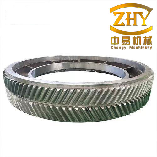
The herringbone gear, formed by two symmetrically arranged helical gears with opposite helix directions, not only inherits the advantages of helical gears such as high load capacity and smooth transmission but also overcomes the drawback of excessive axial forces that accelerate supporting bearing wear in helical gears. It is the preferred gear type for high-speed, heavy-duty, and high-power transmission applications. The study of herringbone gear dynamics has attracted extensive attention from researchers worldwide. The time-varying meshing stiffness, dynamic tooth loads, and the resulting structural vibrations are critical aspects that govern the reliability and acoustic performance of the entire drivetrain.
1. Research Background and Significance
Gear transmission devices are essential mechanisms for transmitting motion and power in modern mechanical equipment, widely used in marine, automotive, aviation, and aerospace industries. Comparing with other mechanical systems, gear systems may exhibit vibrations not only due to external excitations such as input speed fluctuations and load torque variations but also in the absence of external excitation. This is because the elastic deformation of gear teeth and the alternating number of meshing tooth pairs during transmission lead to continuously varying meshing stiffness, generating dynamically changing meshing forces and causing gear vibrations. The time-varying nature of gear meshing stiffness places the gear system in a parametric vibration state, which fundamentally determines the properties of the gear system dynamic model. Therefore, solving and analyzing the meshing stiffness excitation is a prerequisite and essential step for gear dynamics analysis.
Furthermore, gear transmission systems frequently alternate between accelerating startup, constant-speed operation, and decelerating shutdown conditions. Harsh working environments severely affect operational stability. Traditional static gear strength checks relying on approximate calculations and empirical formulas are difficult to meet modern design requirements. To improve dynamic characteristics, load-carrying capacity, and reliability of gear transmission, precisely measuring indicators such as tooth surface load distribution, tooth surface contact dynamic stress, and tooth root bending dynamic stress during dynamic meshing is an important aspect of gear dynamic design.
With the advancement of industrial technology, gearboxes are developing toward higher speeds and heavier loads. The increasing transmission power and rotational speed have made vibration problems increasingly prominent. In the aerospace and marine industries, gear system vibrations generate noise that compromises the stealth capability of aircraft and ships and affects personnel health. In severe cases, this can lead to connected equipment failure and even casualties. Therefore, vibration control research of gearboxes has always been a key focus area, possessing significant engineering practical value and theoretical significance.
2. Gear Dynamics Modeling and Finite Element Contact Analysis Theory
2.1 Basic Theory of Gear System Dynamics
Gear system dynamics is a discipline that studies the dynamic behavior of gear systems during motion and power transmission. Similar to general mechanical systems, the dynamic problems of gear systems can be divided into three fundamental issues: dynamic excitation, system modeling, and dynamic response. The dynamic excitations include both external excitations (such as prime mover torque and load resistance torque) and internal excitations (including time-varying meshing stiffness excitation, gear error excitation, and meshing impact excitation). Building a proper analysis model is the central task of gear system dynamics. Various methods exist for establishing these models, including the lumped parameter method, transfer matrix method, finite element method, and dynamic substructure synthesis method.
The traditional solution process for gear dynamics begins with identifying internal and external excitations. External excitations come from the prime mover and driven load, while internal excitations arise from time-varying stiffness, gear errors, and impact during meshing. A dynamic model is then constructed—ranging from simple single-degree-of-freedom models to complex multi-degree-of-freedom systems that include gears, shafts, bearings, and housing structures. Finally, the dynamic response is solved through numerical integration methods, enabling parameter studies and noise radiation prediction.
2.2 Mathematical Model of Herringbone Gear Transmission
The herringbone gear transmission system examined in this study consists of two symmetrically arranged helical gear pairs with identical geometric and material parameters. Thus, their comprehensive meshing stiffnesses and damping coefficients are essentially equal. Under high manufacturing and assembly precision, axial forces cancel each other, and axial vibration is negligible. Treating the transmission shafts as rigid bodies and considering the symmetry of the model, a half-model of the herringbone gear transmission was adopted for analysis, yielding a six-degree-of-freedom lumped parameter model.
The generalized displacement vector is defined as:
\[
\{\delta\} = \{x_1, y_1, \theta_1, x_2, y_2, \theta_2\}^\mathrm{T}
\]
where x1, x2 and y1, y2 are the translational vibration displacements of the driving and driven gear centers along the x and y directions, respectively, and θ1 and θ2 are the rotational vibration displacements around the z-axis.
Given the normal meshing stiffness km, normal damping cm, and normal comprehensive error e of the helical gear, these quantities can be resolved into the y-direction components:
\[
k_{my} = k_m \cos^2\beta, \quad c_{my} = c_m \cos^2\beta, \quad e_y = e \cos\beta
\]
where β is the helix angle. The dynamic meshing force in the y direction can then be expressed as:
\[
F_y = k_{my}(y_1 + R_{t1}\theta_1 – y_2 + R_{t2}\theta_2 – e_y) + c_{my}(\dot{y}_1 + R_{t1}\dot{\theta}_1 – \dot{y}_2 + R_{t2}\dot{\theta}_2 – \dot{e}_y)
\]
Considering tooth friction, the vibration differential equations of the system can be derived and expressed in matrix form as:
\[
[M]\{\ddot{\delta}\} + [C]\{\dot{\delta}\} + [K]\{\delta\} = \{P\}
\]
where [M], [C], and [K] are the mass, damping, and stiffness matrices, respectively, and {P} is the external force vector. All these matrices were systematically derived and reported in the thesis.
2.3 Contact Dynamics Finite Element Theory
Contact problems are ubiquitous in mechanical engineering, involving three types of nonlinearities: geometric nonlinearity from large deformations, material nonlinearity, and contact interface nonlinearity characteristic of contact problems. In finite element analysis, contact conditions represent a special type of discontinuous constraint. ABAQUS provides both Standard and Explicit modules for contact analysis. In the Standard module, contact pairs or self-contact can be defined with control over normal and tangential behavior. The Explicit module offers general contact algorithms and contact pair algorithms.
Three mathematical methods describe non-penetration constraints: the Lagrange multiplier method, the penalty function method, and the direct constraint method. The penalty function method, widely used in explicit dynamic contact analysis, was employed in this study to handle contact constraints during gear dynamic meshing. This method does not increase the number of unknowns and is numerically straightforward to implement.
3. Numerical Calculation and Analysis of Herringbone Gear Meshing Stiffness
3.1 Basic Concept of Gear Comprehensive Meshing Stiffness
Gear meshing stiffness is defined as the load required to produce 1 μm deformation per 1 mm tooth width on one or several pairs of teeth meshing simultaneously. The comprehensive meshing stiffness of a gear pair is the combined effect of all tooth pairs in simultaneous contact within the meshing zone, primarily related to single-tooth elastic deformation, comprehensive elastic deformation of a single tooth pair, and the contact ratio. The single-tooth elastic deformation includes bending deformation, shear deformation, and contact deformation. For a single tooth pair in mesh, the comprehensive elastic deformation is the sum of the individual tooth deformations. The single-pair meshing stiffness can be expressed as:
\[
k_s = \frac{k_1 k_2}{k_1 + k_2}
\]
where k1 and k2 are the single-tooth stiffnesses of the driving and driven gears, respectively. The comprehensive gear meshing stiffness is the superposition of all meshing tooth pair stiffnesses. For helical gears, the meshing process starts from one end of the tooth, gradually extends to the full tooth surface, and exits from the other end. Consequently, although the meshing stiffness of helical gear teeth is time-varying, it does not exhibit the stepped sudden changes characteristic of spur gears but fluctuates mildly around a certain value.
3.2 Calculation Method for Time-Varying Meshing Stiffness
The herringbone gear can be considered as two helical gears with equal helix angles and opposite helix directions combined in parallel. Therefore, its meshing stiffness can be indirectly calculated from the helical gear stiffness using the parallel relationship. The basic dynamic equation of a single helical gear pair is:
\[
m\ddot{\delta} + c\dot{\delta} + k\delta = F
\]
The meshing stiffness is only related to gear structure, load conditions, and current meshing position, hence:
\[
k = \frac{F}{\delta}
\]
Introducing the concept of transmission error and defining the loaded transmission error (LTE), the loaded transmission error along the line of action can be expressed as:
\[
\mathrm{LTE} = R_{bn2}\theta_2 – R_{bn1}\theta_1
\]
where Rbn1 and Rbn2 are the base circle radii in the normal plane of the driving and driven gears, respectively. The loaded transmission error is further decomposed into the unloaded transmission error (NLTE) and the gear elastic deformation. Consequently, the helical gear meshing stiffness can be written as:
\[
k = \frac{F_n}{\delta} = \frac{F_n}{R_{bn2}\theta_2 – R_{bn1}\theta_1 – \mathrm{NLTE}}
\]
For the herringbone gear, by the parallel connection of two helical gear pairs:
\[
k_m = 2k = \frac{2F_n}{R_{bn2}\theta_2 – R_{bn1}\theta_1 – \mathrm{NLTE}}
\]
3.3 Finite Element Model for Helical Gear Meshing Stiffness
The analyzed herringbone gear is used in a marine reduction gearbox, where the driving wheel inputs a rotational speed and the driven wheel is subjected to a load torque. The basic parameters of the helical gear pair are given in Table 3.1.
| Parameters | Driving gear | Driven gear |
|---|---|---|
| Number of teeth | 31 | 102 |
| Normal module (mm) | 4.5 | 4.5 |
| Pressure angle (°) | 20 | 20 |
| Helix angle (°) | 28.2024 | 28.2024 |
| Face width (mm) | 90 | 90 |
The transverse contact ratio and overlap ratio were calculated as:
\[
\varepsilon_\alpha = 1.46
\]
\[
\varepsilon_\beta = \frac{b \tan\beta}{\pi m_t} = \frac{90 \times \tan 28.2024^\circ}{\pi \times 5.11} \approx 3.00
\]
The total contact ratio is therefore:
\[
\varepsilon_\gamma = \varepsilon_\alpha + \varepsilon_\beta = 1.46 + 3.00 = 4.46
\]
Given the high contact ratio, the meshing tooth pairs vary between four and five. A ten-tooth model was adopted to balance computational efficiency and accuracy. Both crowned and uncrowned (i.e., with and without gear hub) models were created to investigate the influence of the hub structure. Boundary conditions were established by coupling reference points at the gear rotation axes with the inner bore surfaces, with appropriate displacement and force constraints applied to these reference points.
Before proceeding with helical gear analysis, the finite element contact model was validated against Hertz contact theory using a spur gear pair. The maximum contact pressure from Hertz theory is:
\[
p_{\max} = \sqrt{\frac{\frac{1}{R_1} + \frac{1}{R_2}}{\pi L \left( \frac{1-\mu_1^2}{E_1} + \frac{1-\mu_2^2}{E_2} \right)}} \cdot P
\]
The comparison results are shown in Table 3.2.
| Driven gear torque (Nm) | 460 | 560 | 660 | 760 | 860 |
|---|---|---|---|---|---|
| Hertz stress (MPa) | 750.7 | 838.6 | 918.9 | 993.4 | 1063.1 |
| FEA result (MPa) | 707.9 | 795.0 | 874.4 | 932.8 | 1004.6 |
| Relative error (%) | -5.7 | -5.2 | -4.8 | -6.1 | -5.5 |
The relative errors are within 10%, validating the accuracy and effectiveness of the finite element contact model. Using a mesh with a minimum element size of 0.461 mm in the tooth height direction, 0.596 mm in the face width direction, and 0.267 mm in the tooth thickness direction, the model contained 234,538 nodes and 208,164 elements in the validation study.
The helical gear geometry was created in UG software and meshed in Hypermesh to obtain high-quality hexahedral elements. Due to the complex tooth surface geometry, sophisticated splitting operations were required before sweep meshing could be applied. The final mesh model for the helical gear pair is shown in Figure 3.11. In ABAQUS, material properties were defined with an elastic modulus of 209 GPa and Poisson’s ratio of 0.29, using C3D8R elements. A static general analysis was performed with contact pairs defined on potential contacting surfaces. Hard contact for normal behavior and frictionless tangential behavior were specified. The analysis was divided into four steps: establishing contact, applying a small torque, applying the rated torque, and finally driving the gear pair by prescribing rotation.
3.4 Calculation Results of Time-Varying Meshing Stiffness
Using the finite element model and the analysis procedure described above, the transmission error under a rated torque of 3000 Nm was calculated. The unloaded transmission error (using a 15 Nm load approximating no-load) exhibited periodic fluctuations with an average value of 1.35 μm, primarily attributed to geometric and mesh model errors. The loaded transmission error showed a periodic variation with an average value of 10.95 μm. The difference between the loaded and unloaded transmission errors represents the comprehensive elastic deformation under rated load.
Extracting the time history of normal contact forces for each meshing tooth pair, the herringbone gear system alternated between four-tooth and five-tooth meshing zones. From the analysis, the loaded contact ratio was determined to be 4.75, which is 0.29 higher than the unloaded value of 4.46, indicating an increase in effective contact ratio under load due to tooth elastic deformation.
The comprehensive meshing stiffness of the helical gear pair was calculated as:
\[
k = \frac{F}{\mathrm{LTE} – \mathrm{NLTE}}
\]
The resulting stiffness curve exhibited a clear periodic characteristic with a minimum period of 0.12 s. The maximum stiffness was 1.453×10⁹ N/m, occurring at the middle of the five-tooth meshing zone where the load distribution was most uniform. The minimum stiffness was 1.446×10⁹ N/m, occurring at the transition point where one pair just exited and the system entered the four-tooth meshing zone. Due to the high contact ratio, the stiffness fluctuation is small, confirming excellent load-carrying capacity and smooth operation of the herringbone gear. For the full herringbone gear, the stiffness is double that of a single helical half, i.e., approximately 2.9×10⁹ N/m.
3.5 Analysis of Factors Influencing Helical Gear Meshing Stiffness
Three factors were systematically investigated: gear hub, applied load, and elastic modulus.
Influence of gear hub: A gear model without the hub structure was created, maintaining identical geometric, material, and mesh parameters. Although the contact forces were essentially the same, the model without the hub exhibited a loading transmission error of 10.40 μm compared to 10.99 μm for the model with hub—a 5% reduction. The comprehensive stiffness increased from 1.453×10⁹ N/m to 1.627×10⁹ N/m—a 12% increase. This is because the no-hub model inherently neglects hub deformation, equivalent to treating the hub as rigid. Hence, the gear hub cannot be neglected when calculating meshing stiffness.
Influence of load: Five load levels (1 KNm, 1.5 KNm, 2 KNm, 2.5 KNm, 3 KNm) were applied to the model with hub. The loaded transmission error increased linearly with increasing load. The meshing stiffness also increased with load, but the rate of increase gradually diminished. This confirms that load-dependent deformation affects the mesh state and hence the effective stiffness.
Influence of elastic modulus: Four elastic modulus values (5×10⁴ MPa, 1×10⁵ MPa, 1.5×10⁵ MPa, 2×10⁵ MPa) were examined. Larger elastic moduli resulted in smaller transmission errors, consistent with stiffer materials deflecting less under the same load. The meshing stiffness increased approximately linearly with elastic modulus. The relationship between stiffness, load, and elastic modulus is essential for predicting the dynamic behavior of herringbone gear pairs under different operating conditions.
4. Finite Element Analysis of Herringbone Gear Dynamic Meshing Performance
4.1 Explicit Dynamic Contact Finite Element Modeling
The explicit dynamics analysis is based on the central difference method for time integration. The accelerations at time t are used to determine velocities at t+Δt/2, which are then used to compute displacements at t+Δt, expressed as:
\[
\dot{u}_{i+1/2}^N = \dot{u}_{i-1/2}^N + \frac{\Delta t_{i+1} + \Delta t_i}{2}\ddot{u}_i^N
\]
\[
u_{i+1}^N = u_i^N + \Delta t_{i+1} \dot{u}_{i+1/2}^N
\]
The central difference method is only conditionally stable, with the stable time increment estimated from the smallest element dimension and the dilatational wave speed:
\[
\Delta t \approx \frac{L_{\min}}{c_d}
\]
For isotropic linear elastic materials, the dilatational wave speed is expressed as:
\[
c_d = \sqrt{\frac{\hat{\lambda} + 2\hat{\mu}}{\rho}}
\]
where \(\hat{\lambda} = \frac{E\nu}{(1+\nu)(1-2\nu)}\) and \(\hat{\mu} = \frac{E}{2(1+\nu)}\) are the Lamé constants.
Rayleigh damping was employed to represent energy dissipation:
\[
[C] = \alpha[M] + \beta[K]
\]
The critical damping ratio is related to the Rayleigh coefficients by:
\[
\xi_i = \frac{\alpha}{2\omega_i} + \frac{\beta \omega_i}{2}
\]
For the gear dynamic analysis, mass and stiffness proportional coefficients of α = 800 rad/s and β = 5×10⁻⁸ were adopted, corresponding to a damping ratio within the typical 2%–10% range for mechanical systems.
Due to the use of reduced-integration elements, hourglass control was essential. Enhanced hourglass control was employed to prevent zero-energy deformation modes. The mesh model for the herringbone gear dynamic analysis contained 910,084 elements and 1,075,910 nodes, with refined mesh in the eight teeth involved in dynamic meshing analysis.
The material parameters specified in the dynamic simulation are shown in Table 4.1.
| Component | ρ (kg/m³) | E (Pa) | μ |
|---|---|---|---|
| Driving and driven gears | 7.8×10³ | 2.09×10¹¹ | 0.29 |
Kinematic coupling constraints were established between reference points at the gear centers and the inner bore surfaces of the gears. The driving gear was prescribed with a rotational speed n = 1000 rpm while the driven gear was loaded with a resisting torque TL = 6000 Nm. The amplitude curves were applied gradually to avoid severe initial impact.
4.2 Dynamic Meshing Impact Characteristics
Extracting the rotational speed and angular acceleration of both gears during the startup acceleration phase, the driving gear’s stable speed was 104.67 rad/s, corresponding to the applied 1000 rpm, while the driven gear’s stable speed was 31.8 rad/s, satisfying the transmission ratio requirement. During the initial 0.1 ms, due to meshing impact, the angular accelerations of both gears changed dramatically, reaching peak values within approximately 0.5 ms, and then rapidly decaying toward zero because of the relatively high damping. The tooth contact forces of the first five tooth pairs exhibited significant oscillation peaks during the 0-1 ms startup impact region, while the sixth pair, which entered meshing later, was not affected by the startup impact.
4.3 Tooth Surface Contact Region and Dynamic Contact Stress
The contact regions of the left and right halves of the herringbone gear were symmetrically distributed, with essentially identical contact stresses due to geometric symmetry. At time 2.6 ms, five tooth pairs were simultaneously in mesh, and the contact stress values at most locations ranged from 250-300 MPa, with localized peaks of approximately 600 MPa at tooth tips due to stress concentration. At 7.8 ms, four tooth pairs were in mesh, yielding relatively lower load-carrying capacity, with some contact stress values reaching 700 MPa at tooth tips.
To investigate the time-varying contact stress at different positions, four elements (A, B, C, D) on the driving gear tooth surface and four elements (E, F, G, H) on the driven gear were examined. The maximum contact stress values decreased from A to C, consistent with the increasing curvature radius along the tooth profile per Hertz contact theory. The contact stress distribution along the tooth contact line remained relatively uniform, confirming stable contact conditions during meshing.
4.4 Tooth Root Bending Dynamic Stress
Gear teeth act as cantilever beams fixed at the tooth root. The tooth root fillets experience maximum tensile and compressive stresses, making them the most critical regions. Through the dynamic simulation, the bending stress distributions on both halves of the herringbone gear were symmetric and reasonable. At 2.6 ms, the driving gear root stress values were within 140 MPa, and the driven gear values did not exceed 120 MPa. At 7.8 ms, the stress values were slightly higher due to the reduced number of simultaneously engaged tooth pairs.
Examining the time-varying bending stress at different root positions, during the 0-1 ms meshing impact region, the impact root bending stresses were nearly twice the normal stress values. The maximum root bending stresses for the driving and driven gears were 212 MPa and 185 MPa, respectively. For the driving gear, the bending stress increased slowly from zero at the root entry to the maximum, then decreased rapidly at the tooth tip exit. Conversely, for the driven gear, the bending stress increased rapidly at the tip entry and decreased slowly at the root exit. These patterns are consistent with the respective engagement and disengagement processes.
4.5 Influence of System Parameters on Dynamic Meshing Performance
Effect of system damping: Increasing the Rayleigh mass proportionality coefficient α from 400 to 800 rad/s reduced the oscillation amplitudes of the angular speed and angular acceleration curves and accelerated the decay of transient oscillations. The damping coefficient had a negligible influence on the initial startup impact but substantially influenced the residual vibration. Higher damping also produced slightly higher bending stress values at the same time instants while reducing oscillation amplitudes.
Effect of rotational speed: Three speeds were examined: 600, 800, and 1000 rpm. While the steady-state speeds correctly followed the transmission ratio, the peak angular accelerations during the impact phase were larger at higher speeds, indicating more severe meshing impact. The corresponding oscillation amplitudes in the decay phase were also larger, but the decay rate remained essentially unchanged.
Effect of load: Load torques of 6 KNm, 8 KNm, and 10 KNm were investigated. Since the input speed, system damping, and ramp time were identical, the load level had virtually no influence on the rotational speed and angular acceleration curves. However, the tooth root bending stresses increased with increasing load. Notably, the stress increment was not linearly proportional to the load increment; the percentage increase in stress was smaller than the percentage increase in load.
5. Modal Analysis and Vibration Response Analysis of the Gearbox
5.1 Theoretical Basis of Modal Analysis and Modal Superposition Method
Finite element modal analysis is performed by discretizing the continuous structure and solving the eigenvalue problem. For a multi-degree-of-freedom system, the free vibration equation in the absence of damping is:
\[
[M]\{\ddot{\delta}\} + [K]\{\delta\} = 0
\]
Assuming harmonic motion \(\{\delta\} = \{X\}\cos(\omega t + \varphi)\), the eigenvalue problem becomes:
\[
([K] – \omega^2[M])\{X\} = 0
\]
Solving the characteristic equation \(|K – \omega^2 M| = 0\) yields the natural frequencies and mode shapes. The modal superposition method follows by transforming the physical coordinates to modal coordinates. With mass-normalized mode shapes forming the modal matrix [X], the transformation \(\{\delta\} = [X]\{q\}\) decouples the equations of motion into n independent single-degree-of-freedom equations:
\[
\ddot{q}_i(t) + 2\xi_i\omega_i\dot{q}_i(t) + \omega_i^2 q_i(t) = Q_i(t)
\]
where Qi(t) is the modal force, and ξi is the modal damping ratio, obtained from Rayleigh damping coefficients. This approach significantly reduces computational effort compared to direct time integration when a sufficient number of modes is retained.
5.2 Modal Analysis of the Gear Transmission System
The finite element models of the driving shaft and driven shaft were created in Hypermesh. In ABAQUS, reference points were established at the bearing centers and coupled to the bearing bore surfaces. Bearings were simulated by constraining all degrees of freedom of the reference points except rotation about the shaft axis. The Lanczos eigensolver was used to extract the first ten natural frequencies and mode shapes.
For the driving shaft, the first mode had zero frequency corresponding to rigid-body rotation about the z-axis, which is physically consistent since the axial rotational degree of freedom was not constrained. Several pairs of nearly identical frequencies were observed due to the axisymmetric structure. The natural frequencies ranged from 1462.5 Hz to 2799.7 Hz for the first ten modes, with mode shapes including local expansion, local bending, transverse bending, and complex local deformation patterns.
For the driven shaft, the first ten natural frequencies were considerably lower, below 1000 Hz. This is because the driven gear has a larger mass and significant portions of its hub were removed for weight reduction, decreasing overall stiffness. The mode shapes included local rotation, local expansion, transverse bending, and complex deformation.
The natural frequencies and mode shape descriptions for both shafts are summarized in Tables 5.1 and 5.2.
| Mode | Frequency (Hz) | Description |
|---|---|---|
| 1 | 0 | Rigid rotation about Z axis |
| 2 | 1462.5 | Local expansion |
| 3 | 1511.3 | Local bending |
| 4 | 1511.3 | Local bending |
| 5 | 2163.6 | Local expansion/contraction |
| 6 | 2219.9 | Transverse bending |
| 7 | 2220.0 | Transverse bending |
| 8 | 2522.0 | Complex local deformation |
| 9 | 2522.5 | Complex local deformation |
| 10 | 2799.7 | Local rotation |
| Mode | Frequency (Hz) | Description |
|---|---|---|
| 1 | 0 | Rigid rotation about Z axis |
| 2 | 238.55 | Local rotation |
| 3 | 238.60 | Local rotation |
| 4 | 506.86 | Local expansion/contraction |
| 5 | 567.29 | Transverse bending |
| 6 | 567.95 | Transverse bending |
| 7 | 741.93 | Local expansion |
| 8 | 899.20 | Local bending |
| 9 | 899.20 | Local bending |
| 10 | 916.22 | Complex deformation |
5.3 Modal Analysis of the Gearbox Housing
The gearbox housing was modeled in Hypermesh with detailed geometry simplification and high-quality hexahedral mesh generation. The housing material was HT300 gray cast iron with material parameters given in Table 5.3.
| Material | ρ (kg/m³) | E (Pa) | μ |
|---|---|---|---|
| HT300 | 7.3×10³ | 1.3×10¹¹ | 0.25 |
The upper and lower housing parts were connected by bonded contact simulating bolted connections, and the bolt holes at the base were fully constrained. The first ten natural frequencies and mode shapes were extracted, as listed in Table 5.4.
| Mode | Frequency (Hz) | Description |
|---|---|---|
| 1 | 188.2 | Ventilation hole motion |
| 2 | 259.13 | Swing in Z direction |
| 3 | 264.12 | Expansion and contraction |
| 4 | 313.68 | Top plate distortion |
| 5 | 359.68 | Upper housing motion in Z |
| 6 | 385.47 | Contraction deformation |
| 7 | 389.43 | Compression deformation |
| 8 | 406.01 | Upper side wall twisting |
| 9 | 420.37 | Side wall and top distortion |
| 10 | 433.87 | Twisting and Z swing |
All ten natural frequencies were below 500 Hz, reflecting the relatively flexible nature of the housing structure. The mode shapes predominantly involved deformation of the upper housing, while the lower housing remained nearly undeformed in the low-frequency range due to its base being fixed.
5.4 Extraction of Bearing Excitation Forces
The key to analyzing gearbox housing vibration is accurately extracting the dynamic forces transmitted through the bearings. A multi-body dynamics model of the herringbone gear transmission system was established in ADAMS software. The gear meshing stiffness was set to 2.9×10⁶ N/mm based on the finite element calculation, with a contact force exponent of 1.5, damping coefficient of 30 N·s/mm, and a damping penetration depth of 0.05 mm. Friction was modeled with static and dynamic friction coefficients of 0.3 and 0.1, respectively.
The simulation was performed with an input speed of 1000 rpm and a load torque of 6000 Nm. Due to the transient nature of the initial startup phase, only the steady-state data from 0.04 s to 0.06 s (200 data points) were extracted for further analysis. The bearing reaction forces on both the driving and driven shaft bearings exhibited periodic variations. The average bearing forces on the driving shaft were larger than those on the driven shaft due to the smaller pitch radius of the driving gear, although the torques were approximately equal.
The frequency spectrum of the bearing forces showed distinct peaks at the gear meshing frequency and its harmonics. The theoretical gear meshing frequency is given by:
\[
f_m = \frac{n \cdot z}{60} = \frac{1000 \times 31}{60} \approx 516 \ \mathrm{Hz}
\]
The agreement between the simulation results and theoretical calculations validated the multi-body dynamics model and the extracted bearing forces.
5.5 Vibration Response Analysis of the Gearbox Housing
Using the modal superposition method, the vibration response of the gearbox housing was computed by applying the bearing forces as excitation at the bearing housing locations. The first 20 modes of the housing were extracted, and a transient modal analysis step was established in ABAQUS. The horizontal and vertical bearing force components were applied as analytical field functions at the corresponding bearing support locations, with fixed constraints at the base bolt holes.
The stress distribution contours of the gearbox at times 0.045 s and 0.05 s revealed that the connections between stiffening ribs and the housing side walls, along with the base bolt holes, were the weakest locations. The stiffening ribs, designed to enhance vertical stiffness, are located near the bearing supports and withstand a significant portion of the bearing reaction forces.
To examine the vibration response of surface nodes, two reference points were selected: Point A at the bearing housing of the driving shaft input end and Point B at the bearing housing of the driven shaft output end. The vibration displacement, velocity, and acceleration time-history curves were extracted in both the x and y directions.
Because the bearing forces on the driving shaft were larger, the vibration magnitudes (displacement, velocity, and acceleration) at Point A were consistently larger than those at Point B. Moreover, due to the stiffening effect of the ribs, the y-direction stiffness of the gearbox was larger than the x-direction stiffness, so the vibration values in the x direction were larger than those in the y direction for the same reference point.
The frequency-domain analysis of the displacement showed that the peak amplitude occurred at the gear meshing frequency of approximately 516 Hz, confirming that the gearbox vibration response is most pronounced at the meshing frequency. This finding is crucial for vibration control: reducing the dynamic excitation at the source, such as optimizing the herringbone gear meshing stiffness, is the most direct approach to mitigating gearbox vibration.
The displacement amplitude spectra also indicated secondary peaks at the harmonics of the meshing frequency, although at significantly lower magnitudes. The displacement values observed were on the order of micrometers, with the maximum displacement in the x direction at Point A reaching approximately 0.6 μm, while the corresponding y direction maximum was around 0.3 μm. The velocity and acceleration responses exhibited dominant frequency components consistent with the meshing frequency.
6. Conclusions and Perspectives
This study focused on the dynamic simulation of a herringbone gear transmission system and the vibration response analysis of its gearbox. The main conclusions and achievements are summarized as follows:
(1) A six-degree-of-freedom lumped parameter mathematical model of the herringbone gear transmission system was established, incorporating gear transmission error, comprehensive meshing stiffness, and meshing damping as excitation parameters. The governing equations were formulated in matrix form, providing a theoretical foundation for subsequent analyses.
(2) The Hertz contact theory validated the accuracy of the finite element static contact approach. A systematic investigation of the herringbone gear meshing stiffness was performed using the finite element method. The results confirmed that ignoring the gear hub leads to a 12% overestimation of meshing stiffness, demonstrating that the gear hub cannot be neglected. The meshing stiffness increases with increasing load but with a diminishing rate of increase, and the stiffness is linearly proportional to the elastic modulus. These findings provide quantitative guidance for stiffness prediction under varying operating conditions.
(3) The explicit dynamic contact finite element model of the herringbone gear was established. The dynamic meshing performance during the startup acceleration phase was simulated, revealing significant impact forces during the initial 0.1-0.5 ms. The tooth surface contact stress and tooth root bending stress distributions were obtained, identifying the critical locations. Parametric studies showed that increasing system damping effectively suppresses vibration oscillations; higher rotational speeds intensify meshing impact; and higher loads increase tooth root bending stresses but with a smaller percentage increase.
(4) The modal analyses of the driving shaft, driven shaft, and gearbox housing provided natural frequencies and mode shapes essential for dynamic analysis. The multi-body dynamics simulation of the herringbone gear transmission system yielded bearing reaction forces validated by the agreement between the simulated frequency spectrum and the theoretical meshing frequency. The modal superposition method was then applied to compute the gearbox housing vibration response. The results showed that the stiffening rib connections and base bolt holes are the most vulnerable locations, and the vibration response peaks at the gear meshing frequency.
Future work should focus on several aspects. First, the parametric modeling and solving of herringbone gear meshing stiffness could be developed, enabling rapid evaluation when gear parameters change without remeshing. Second, the multi-body dynamics model could be enhanced by incorporating flexible gear bodies to capture the coupled effects of structural deformation and gear dynamics more accurately. Third, acoustic analysis using finite element or boundary element methods could extend the vibration response analysis to predict radiated noise, supporting comprehensive vibration and noise control design of herringbone gear transmission systems.
In summary, this thesis contributed to the prediction of the dynamic characteristics of herringbone gear transmission systems under specific operating conditions through systematic studies of meshing stiffness, dynamic meshing performance, and gearbox vibration response. The findings provide valuable guidance for the dynamic design and vibration control of herringbone gear systems in practical engineering applications.