
I have focused my research on the dynamic behavior of helical gear transmission systems because these components are widely used in high-speed and heavy-load machinery, such as wind turbines, rail vehicle gearboxes, and industrial reducers. In my work, I treat the helical gear pair as a nonlinear dynamic system influenced by time-varying meshing stiffness, time-varying friction, stick-slip transitions, and progressive tooth surface wear. I establish several coupled models and then solve them numerically to reveal how friction-induced stick-slip and wear alter the vibration response of the helical gear system.
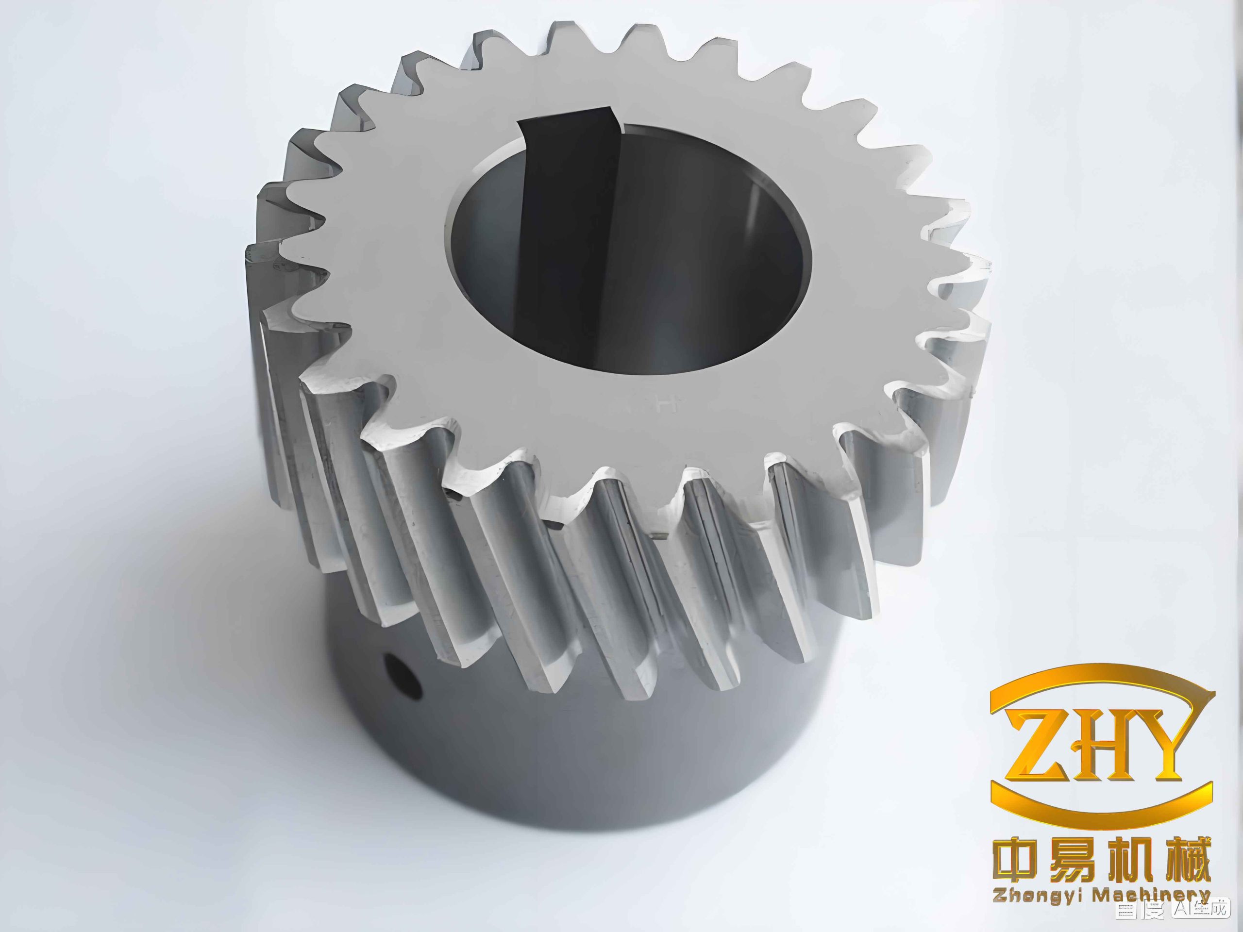
My analysis begins with the time-varying meshing characteristics of a helical gear pair. I calculate the contact line length, the friction coefficient, and the meshing force as functions of rotation angle, load, and speed. I then incorporate these quantities into a dynamic model with eight degrees of freedom. The influence of stick-slip friction is introduced through a transition condition that switches the contact state between sliding and adhesion. After that, I develop a wear model based on the Archard equation and simulate the wear depth on both driving and driven helical gear teeth. Finally, I perform modal analysis and dynamic response analysis to quantify how wear changes natural frequencies, mode shapes, harmonic content, phase trajectories, and Poincaré maps.
Time-Varying Meshing Characteristics of the Helical Gear Pair
For a helical gear pair, the contact line is inclined relative to the tooth width because of the helix angle. This geometry makes the meshing process gradual: contact lines enter and leave the meshing zone continuously, and the total contact line length changes with the rotation angle. I divide the meshing zone into six regions according to the position of the contact line relative to the pitch line. When the transverse contact ratio is larger than the axial contact ratio, the lengths on the two sides of the pitch line can be expressed as follows:
$$ a_1 = \frac{s_i}{\sin \beta_b}, \quad a_2 = 0, \quad \text{for } 0 \le s_i < \frac{l_1}{\sin \beta_b} $$
$$ a_1 = \frac{l_1}{\sin \beta_b}, \quad a_2 = \frac{s_i – l_1}{\sin \beta_b}, \quad \text{for } \frac{l_1}{\sin \beta_b} \le s_i < \frac{P_{bt}}{\sin \beta_b} $$
$$ a_1 = \frac{P_{bt} – s_i}{\sin \beta_b}, \quad a_2 = \frac{s_i – l_1}{\sin \beta_b}, \quad \text{for } \frac{P_{bt}}{\sin \beta_b} \le s_i < \frac{P_{bt} + l_1}{\sin \beta_b} $$
$$ a_1 = \frac{P_{bt} – s_i}{\sin \beta_b}, \quad a_2 = \frac{l_2}{\sin \beta_b}, \quad \text{for } \frac{P_{bt} + l_1}{\sin \beta_b} \le s_i < \frac{P_{bt} + l_2}{\sin \beta_b} $$
$$ a_1 = 0, \quad a_2 = \frac{l_m – s_i + P_{bt}}{\sin \beta_b}, \quad \text{for } \frac{P_{bt} + l_2}{\sin \beta_b} \le s_i < \frac{P_{bt} + l_m}{\sin \beta_b} $$
$$ a_1 = 0, \quad a_2 = 0, \quad \text{for } \frac{P_{bt} + l_m}{\sin \beta_b} \le s_i < N P_{bt} + l_m $$
Here, \(a_1\) and \(a_2\) are the contact line lengths on the left and right sides of the pitch line, \(s_i\) is the distance traveled by the \(i\)-th tooth pair after entering the meshing zone, \(P_{bt}\) is the base transverse pitch, \(\beta_b\) is the base helix angle, \(l_1\) and \(l_2\) are the distances from the initial and final meshing positions to the pitch line, and \(l_m\) is the actual length of the line of action. The total contact line length is \(L = a_1 + a_2\). The contact ratio components are:
$$ \varepsilon_\alpha = \frac{L}{P_{bt}}, \quad \varepsilon_\beta = \frac{b \tan \beta_b}{P_{bt}}, \quad \varepsilon = \varepsilon_\alpha + \varepsilon_\beta $$
where \(b\) is the tooth width and \(\varepsilon\) is the total contact ratio. I use these expressions to evaluate how helix angle and tooth width affect the excitation. For the friction coefficient, I apply a regression formula that accounts for Hertzian contact pressure, sliding-to-rolling ratio, entrainment velocity, lubricant viscosity, equivalent curvature radius, and surface roughness. The general form is:
$$ \mu = e^{b_1} P_h^{b_2} |SR|^{b_3} V_e^{b_4} \nu_0^{b_5} R^{b_6} S^{b_7} $$
where \(P_h\) is the maximum Hertzian contact pressure, \(SR\) is the slide-to-roll ratio, \(V_e\) is the entrainment velocity, \(\nu_0\) is the dynamic viscosity of the lubricant, \(R\) is the equivalent curvature radius, \(S\) is the composite root-mean-square roughness, and \(b_1\) to \(b_7\) are regression coefficients. The maximum Hertzian pressure is computed from:
$$ P_h = \sqrt{\frac{F_n E’}{\pi R L}} $$
in which \(F_n\) is the normal meshing force, \(E’\) is the equivalent elastic modulus, and \(L\) is the contact line length. I calculate the sliding velocity, rolling velocity, and slide-to-roll ratio at each contact point along the line of action. The relative sliding velocity vanishes at the pitch point, so the friction coefficient approaches zero there. Near the pitch point, the equivalent curvature radius increases and the sliding velocity decreases, which reduces the friction coefficient. Away from the pitch point, the curvature radius decreases and the sliding velocity increases, which raises the friction coefficient.
Table 1 lists the basic parameters of the helical gear pair I used in my simulations. These values represent a typical high-speed rail gearbox application.
| Parameter | Value |
|---|---|
| Number of teeth, \(Z_1/Z_2\) | 29/69 |
| Normal module, \(m_n\) (mm) | 7 |
| Pressure angle, \(\alpha_n\) (deg) | 26 |
| Helix angle, \(\beta_b\) (deg) | 20 |
| Center distance, \(a\) (mm) | 363 |
| Tooth width, \(b\) (mm) | 70 |
| Young’s modulus, \(E\) (GPa) | 206 |
| Poisson’s ratio, \(\nu\) | 0.3 |
| Surface roughness, \(S\) (\(\mu\)m) | 1.13 |
| Lubricant dynamic viscosity, \(\nu_0\) (Pa·s) | \(13.5 \times 10^{-3}\) |
Using the above parameters, I studied the influence of helix angle and tooth width on the time-varying excitation. As the helix angle increases, the total contact line length decreases, while the axial contact ratio increases and the transverse contact ratio decreases. The total contact ratio still rises because the increase in axial contact ratio is larger than the decrease in transverse contact ratio. The maximum single-tooth friction force decreases with increasing helix angle because the contact area becomes larger and the contact stress is distributed more uniformly. The phase at which the maximum friction force occurs also shifts because the load transmission path and contact zone distribution change with helix angle. When the tooth width increases, the total contact line length increases, the axial contact ratio rises, and the transverse contact ratio remains unchanged. The single-tooth friction force gradually decreases because the load is distributed over a longer contact line, reducing the load per unit length. The maximum friction force phase shifts slightly as the tooth width changes.
Table 2 summarizes the trends I observed for the helical gear pair.
| Parameter | Total contact line length | Axial contact ratio | Transverse contact ratio | Maximum single-tooth friction |
|---|---|---|---|---|
| Helix angle increases | Decreases | Increases | Decreases | Decreases |
| Tooth width increases | Increases | Increases | Unchanged | Decreases |
Stick-Slip Friction Dynamics of the Helical Gear Pair
To capture the coupled effects of time-varying meshing stiffness, time-varying friction, and stick-slip behavior, I established an eight-degree-of-freedom dynamic model for the helical gear pair. Each gear has translational degrees of freedom in the \(x\), \(y\), and \(z\) directions and a rotational degree of freedom about the \(z\)-axis. The equations of motion can be written as:
$$ m_1 \ddot{x}_1 + K_{x1} x_1 + c_{x1} \dot{x}_1 = f_p $$
$$ m_2 \ddot{x}_2 + K_{x2} x_2 + c_{x2} \dot{x}_2 = -f_g $$
$$ m_1 \ddot{y}_1 + K_{y1} y_1 + c_{y1} \dot{y}_1 = -F_n \cos \beta_b $$
$$ m_2 \ddot{y}_2 + K_{y2} y_2 + c_{y2} \dot{y}_2 = F_n \cos \beta_b $$
$$ m_1 \ddot{z}_1 + K_{z1} z_1 + c_{z1} \dot{z}_1 = -F_n \sin \beta_b $$
$$ m_2 \ddot{z}_2 + K_{z2} z_2 + c_{z2} \dot{z}_2 = F_n \sin \beta_b $$
$$ I_1 \ddot{\theta}_1 = T_1 – F_n \cos \beta_b r_{b1} + M_p $$
$$ I_2 \ddot{\theta}_2 = -T_2 + F_n \cos \beta_b r_{b2} – M_g $$
Here, \(m_i\) and \(I_i\) are the mass and moment of inertia of gear \(i\), \(K_{xi}\), \(K_{yi}\), \(K_{zi}\) are the support stiffnesses, \(c_{xi}\), \(c_{yi}\), \(c_{zi}\) are the support damping coefficients, \(F_n\) is the normal meshing force, \(f_p\) and \(f_g\) are the time-varying friction forces on the driving and driven gears, \(M_p\) and \(M_g\) are the friction torques, \(T_1\) is the input torque, \(T_2\) is the load torque, and \(r_{b1}\), \(r_{b2}\) are the base radii. The normal meshing force is:
$$ F_n = K_m(t) \delta + C_m(t) \dot{\delta} $$
where \(K_m(t)\) is the time-varying meshing stiffness, \(C_m(t)\) is the meshing damping, and \(\delta\) is the relative deformation along the line of action:
$$ \delta = (y_1 – y_2) \cos \beta_b + (r_{b1} \theta_1 – r_{b2} \theta_2) \cos \beta_b + (z_1 – z_2) \sin \beta_b – e(t) $$
I calculate the time-varying meshing stiffness using the potential energy method. For a single tooth pair, the total compliance is the sum of Hertzian contact compliance, bending compliance, shear compliance, axial compression compliance, and fillet foundation compliance. The single-tooth stiffness is:
$$ k = \left( \frac{1}{k_h} + \frac{1}{k_{b1}} + \frac{1}{k_{b2}} + \frac{1}{k_{s1}} + \frac{1}{k_{s2}} + \frac{1}{k_{a1}} + \frac{1}{k_{a2}} + \frac{1}{k_{f1}} + \frac{1}{k_{f2}} \right)^{-1} $$
For a helical gear, I use the slice method. The helical gear is equivalent to a series of thin spur gear slices along the tooth width. The total meshing stiffness at any instant is the sum of the stiffnesses of all slices in the meshing zone:
$$ K_m(t) = \sum_{j=1}^{N_s} k_j(t) $$
where \(N_s\) is the number of slices and \(k_j(t)\) is the stiffness of the \(j\)-th slice. This approach produces a smoother stiffness curve for a helical gear than for a spur gear. The helical gear has multiple teeth in contact simultaneously, so the stiffness fluctuation is smaller and the load distribution is more uniform.
The stick-slip transition condition is derived from the relative sliding velocity at the contact point. The relative sliding velocity is:
$$ v_{M2M1} = \left( v_2 \sin \alpha_2 – \dot{x}_2 \right) – \left( v_1 \sin \alpha_1 – \dot{x}_1 \right) $$
where \(v_1\) and \(v_2\) are the tangential velocities of the driving and driven gears, \(\alpha_1\) and \(\alpha_2\) are the pressure angles at the contact point, and \(\dot{x}_1\), \(\dot{x}_2\) are the vibration velocities in the direction perpendicular to the line of action. When \(v_{M2M1} = 0\) and the sliding force is less than the maximum static friction force, the contact enters the stick state. The condition is:
$$ v_{M2M1} = 0, \quad f_{\text{stick}} < \mu f_n $$
In the stick state, the friction force is determined by the elastic deformation of the contact interface and the gear body motion. I express the stick force as:
$$ f_{\text{stick}} = m_1 \ddot{x}_1 + K_{x1} x_1 + c_{x1} \dot{x}_1 = -\left( m_2 \ddot{x}_2 + K_{x2} x_2 + c_{x2} \dot{x}_2 \right) $$
I compared the sliding-only model with the stick-slip model. In the sliding-only model, the friction force direction reverses only once at the pitch point. In the stick-slip model, the relative velocity can reverse several times near the pitch point because of the vibration velocity. I observed that within one meshing period, the contact can enter the stick state up to four times near the pitch point. The stick state occurs more frequently at higher speeds, and the duration of each stick state increases with load. Under high-speed and heavy-load conditions, the helical gear pair is more prone to adhesion. The stick-slip phenomenon causes intense oscillations in the meshing force and friction force. For a single tooth, the meshing force can fluctuate between 10 kN and 150 kN when stick-slip is considered. The friction force in the stick state equals the force required to break the adhesion, and it transitions between stick and slip states repeatedly.
Table 3 compares the sliding-only and stick-slip models for the helical gear pair.
| Feature | Sliding-only model | Stick-slip model |
|---|---|---|
| Relative velocity at pitch point | Zero once per mesh | Zero multiple times, up to four per cycle |
| Friction force direction | Reverses once at pitch point | Reverses repeatedly near pitch point |
| Meshing force fluctuation | Moderate | Severe, 10–150 kN for single tooth |
| Effect of speed | Minor | Stick frequency increases with speed |
| Effect of load | Minor | Stick duration increases with load |
| Adhesion probability | Not considered | High under high speed and heavy load |
Tooth Surface Wear Model and Simulation
I model tooth surface wear using the Archard wear equation. The wear depth at a point \(q\) on the tooth surface after \(n\) load cycles is:
$$ h_q = \int_0^s k p \, ds $$
where \(k\) is the wear coefficient, \(p\) is the contact pressure, and \(s\) is the relative sliding distance. For numerical simulation, I use the incremental form:
$$ h_{q,n} = h_{q,n-1} + k p_{q,n-1} S_p $$
where \(h_{q,n}\) is the wear depth after \(n\) cycles, \(h_{q,n-1}\) is the wear depth after the previous cycle, \(p_{q,n-1}\) is the contact pressure at the same point, and \(S_p\) is the sliding distance per cycle. The contact pressure is calculated from the Hertzian contact model:
$$ a_h = \sqrt{\frac{4 F_n}{\pi b E’} \rho} $$
$$ p = \frac{2 F_t}{\pi a_h l} $$
Here, \(a_h\) is the Hertzian contact half-width, \(F_n\) is the normal force, \(F_t\) is the tangential force, \(b\) is the tooth width, \(\rho\) is the equivalent radius of curvature, \(E’\) is the equivalent elastic modulus, and \(l\) is the contact line length. The sliding distances for the driving and driven gears are:
$$ S_p = a_h \frac{u_p – u_g}{u_p}, \quad S_g = a_h \frac{u_p – u_g}{u_g} $$
where \(u_p\) and \(u_g\) are the tangential velocities of the driving and driven gears at the contact point. The sliding coefficients are:
$$ \lambda_p = \frac{|S_p|}{S_p + S_g}, \quad \lambda_g = \frac{|S_g|}{S_p + S_g} $$
I simulated the wear process for the helical gear pair with the parameters in Table 1. The input torque was 2000 N·m, and the driving gear speed was 1500 r/min. Table 4 lists the wear simulation parameters.
| Parameter | Value |
|---|---|
| Number of teeth, \(Z_1/Z_2\) | 29/69 |
| Normal module, \(m_n\) (mm) | 7 |
| Pressure angle, \(\alpha_n\) (deg) | 26 |
| Helix angle, \(\beta_b\) (deg) | 20 |
| Tooth width, \(b\) (mm) | 70 |
| Input torque, \(T_p\) (N·m) | 2000 |
| Driving gear speed, \(n_1\) (r/min) | 1500 |
| Load cycles, \(N\) | \(8 \times 10^7\) |
The contact pressure distribution along the line of action is not uniform. In the double-tooth meshing zone, only two teeth share the load, so the contact pressure is higher. In the triple-tooth meshing zone, three teeth share the load, so the contact pressure is lower. Therefore, the average contact pressure is higher in the middle of the meshing zone and lower at the beginning and end. The sliding coefficient and sliding distance show a V-shaped distribution. At the tooth root, the sliding coefficient reaches a maximum. At the tooth tip, the sliding coefficient is relatively lower. At the pitch point, the sliding coefficient is zero because there is pure rolling. The driving gear has a higher sliding coefficient than the driven gear. The sliding distance follows the same trend as the sliding coefficient. From the tooth root to the tooth tip, the sliding distance first decreases and then increases. At the pitch point, the sliding distance is zero.
After \(8 \times 10^7\) cycles, the wear depth on the driving gear is significantly larger than that on the driven gear. The maximum wear depth occurs near the tooth root in the meshing zone. The wear depth at the tooth root and tooth tip is much larger than that near the pitch point. This is because the relative sliding distance is longer at the root and tip, while the pitch point experiences pure rolling and almost no sliding. I also studied the effects of helix angle, tooth width, input torque, and load cycles on wear depth. The results are summarized in Table 5.
| Parameter | Trend | Reason |
|---|---|---|
| Helix angle increases | Wear depth decreases | Contact line length increases, load per unit length decreases, contact pressure becomes more uniform |
| Tooth width increases | Wear depth decreases | Contact area increases, load per unit length decreases, contact pressure decreases |
| Input torque increases | Wear depth increases | Normal load increases, contact pressure increases, friction and wear accelerate |
| Load cycles increase | Wear depth increases | Plastic deformation accumulates, fatigue damage grows, wear depth accumulates |
The wear depth distribution is a V-shaped curve along the line of action. The minimum wear depth occurs at the pitch point. The maximum wear depth occurs at the tooth root for the driving gear and at the tooth tip for the driven gear. Because the driving gear has fewer teeth, it experiences more cycles in the same time, so its wear depth is larger than that of the driven gear.
Modal Characteristics of the Helical Gear under Wear
I performed modal analysis to study how tooth surface wear affects the natural frequencies and mode shapes of the helical gear system. The general dynamic equation is:
$$ [M]\{\ddot{x}\} + [C]\{\dot{x}\} + [K]\{x\} = \{f(t)\} $$
For free vibration, I neglect damping and external forces, giving:
$$ [M]\{\ddot{x}\} + [K]\{x\} = \{0\} $$
The characteristic equation is:
$$ \det([K] – \omega^2 [M]) = 0 $$
The square roots of the eigenvalues are the natural frequencies \(\omega_1, \omega_2, \dots, \omega_8\). The corresponding eigenvectors are the mode shapes. I used the Block Lanczos method in a finite element simulation. The gear model was meshed with tetrahedral elements. The mesh had 255,374 nodes and 167,657 elements. The average element quality was 0.88. The gear was fixed at the inner bore to simulate an interference fit on the shaft. I extracted the first eight modes. Table 6 shows the natural frequencies before and after wear.
| Mode order | Undamaged frequency (Hz) | Worn frequency (Hz) | Change (%) |
|---|---|---|---|
| 1 | 217.92 | 236.97 | +8.74 |
| 2 | 346.53 | 364.12 | +5.08 |
| 3 | 598.66 | 607.75 | +1.52 |
| 4 | 695.38 | 700.60 | +0.75 |
| 5 | 1124.60 | 1132.20 | +0.68 |
| 6 | 1477.80 | 1482.30 | +0.30 |
| 7 | 2325.00 | 2376.30 | +2.21 |
| 8 | 2619.40 | 2631.10 | +0.45 |
I also calculated the natural frequencies using a lumped-parameter model in MATLAB. The values were 240.78 Hz, 370.57 Hz, 610.84 Hz, 720.43 Hz, 1500.54 Hz, 1600.23 Hz, 2400.68 Hz, and 2650.35 Hz for modes one to eight. The finite element results are slightly lower than the MATLAB results because the finite element model includes more flexibility. The wear-induced changes are more significant for higher-order modes. I observed a sudden jump between the sixth and seventh modes. The increase in the seventh and eighth natural frequencies is much larger than that of the lower modes. This is because higher-order modes are more sensitive to local stiffness changes caused by wear. However, the mode shapes themselves do not change significantly with wear. The first mode is a folding-type vibration. The second mode is a swing-type vibration about the \(Y\)-axis. The third mode is a ring-type vibration about the \(Z\)-axis. The fourth mode is a more complex folding vibration. The fifth and sixth modes are second-order axial folding vibrations. The seventh and eighth modes are third-order folding vibrations. In the radial and folding modes, the deformation of the gear teeth and rim is much larger than that of other parts. This indicates that local deformation becomes more important in higher-order modes.
Dynamic Response of the Helical Gear System under Wear
Wear changes the internal excitations of the helical gear system. The three main internal excitations are stiffness excitation, error excitation, and meshing impact excitation. Wear reduces the meshing stiffness and increases the transmission error. I considered four components of the transmission error: long-period error, short-period error, wear-induced error, and random error. The total error is:
$$ e(t) = e_L + e_S + e_{ms} + e_{\text{random}} $$
The long-period and short-period errors are modeled as sinusoidal functions:
$$ e_L = F_i’ \sin(2\pi f_p t), \quad e_S = f_i’ \sin(2\pi f_m t) $$
where \(F_i’\) is the total tangential composite deviation, \(f_i’\) is the single-tooth tangential composite deviation, \(f_p\) is the rotational frequency, and \(f_m\) is the meshing frequency. The wear-induced error is:
$$ e_{ms} = \min(h_{pi}, h_{gi}) $$
where \(h_{pi}\) and \(h_{gi}\) are the wear depths of the driving and driven gears for the \(i\)-th meshing tooth pair. The random error is \(e_{\text{random}} = 0.2 \times \text{rand}()\). I calculated the static transmission error before and after wear. The amplitude after wear was about 1.5 times the initial amplitude. I also calculated the meshing stiffness after wear. The single-tooth stiffness decreases as wear increases. The total meshing stiffness decreases in both the double-tooth and triple-tooth meshing zones. The reduction in the triple-tooth zone is larger than that in the double-tooth zone because the total wear in the triple-tooth zone is the sum of three teeth.
I analyzed the dynamic response of the driving gear in the \(y\)-direction because my previous results showed that the \(y\)-direction vibration is dominant. I used time-domain analysis, FFT spectrum analysis, phase diagram analysis, and Poincaré map analysis. Table 7 summarizes the dynamic states at different wear cycles.
| Wear cycles | Time-domain amplitude | FFT spectrum | Phase diagram | Poincaré map | Dynamic state |
|---|---|---|---|---|---|
| 0 (undamaged) | Low | Discrete lines at meshing frequency | Closed curve | Single point | Periodic |
| \(2 \times 10^7\) | Moderate | Higher harmonics and sidebands appear | Thickened closed curve | Multiple points | Quasi-periodic |
| \(8 \times 10^7\) | High | Broadened sidebands and continuous bands | Diffuse trajectory band | Distributed point set | Chaotic tendency |
In the undamaged state, the FFT spectrum is dominated by the meshing frequency and its harmonics. The phase diagram is a closed curve, and the Poincaré map shows a single point. This indicates a periodic motion. As wear increases, the amplitude in the time domain grows. The FFT spectrum shows that the amplitudes of the meshing frequency and its harmonics increase. Sidebands appear around the harmonics at intervals of the rotational frequency. The sidebands become wider and more numerous as wear progresses. The phase diagram becomes a thickened closed curve, and the Poincaré map changes from a single point to a set of multiple points. This indicates a transition from periodic to quasi-periodic motion. At the highest wear level, the phase trajectory becomes diffuse, and the Poincaré map shows a distributed set of points. The system tends toward chaotic behavior. These results show that tooth surface wear significantly changes the dynamic response of the helical gear system. The vibration amplitude increases, the frequency content becomes richer, and the motion becomes more complex. The wear-induced changes in stiffness and transmission error are the main causes of this transition.
Conclusion
I have presented a comprehensive study of the dynamic characteristics of helical gears under stick-slip friction and wear effects. The main findings are as follows.
First, the time-varying meshing characteristics of the helical gear are strongly influenced by the helix angle and tooth width. Increasing the helix angle reduces the total contact line length, increases the axial contact ratio, and decreases the maximum single-tooth friction. Increasing the tooth width increases the total contact line length and the axial contact ratio, while the transverse contact ratio remains unchanged. The single-tooth friction decreases because the load is distributed over a longer contact line.
Second, the stick-slip model reveals that the helical gear pair can enter the stick state multiple times near the pitch point. The stick state occurs more frequently at higher speeds and lasts longer under higher loads. The meshing force and friction force fluctuate more severely in the stick-slip model than in the sliding-only model. The stick-slip phenomenon is more likely under high-speed and heavy-load conditions.
Third, the Archard wear model shows that the wear depth on the helical gear teeth follows a V-shaped distribution. The wear depth is minimum at the pitch point and maximum at the tooth root and tooth tip. The driving gear wears more than the driven gear because it experiences more cycles. Increasing the helix angle or tooth width reduces the wear depth, while increasing the input torque or the number of load cycles increases the wear depth.
Fourth, modal analysis shows that wear changes the natural frequencies of the helical gear system, especially the higher-order frequencies. The mode shapes do not change significantly, but the local deformation of the teeth and rim becomes more important in higher-order modes. The finite element results are slightly lower than the lumped-parameter results because of additional flexibility in the finite element model.
Fifth, the dynamic response of the helical gear system changes from periodic to quasi-periodic and then to chaotic as wear progresses. The vibration amplitude increases, the FFT spectrum becomes richer with harmonics and sidebands, the phase diagram thickens, and the Poincaré map changes from a single point to a distributed set. These changes are caused by the wear-induced reductions in meshing stiffness and increases in transmission error.
Overall, my study shows that stick-slip friction and wear have significant effects on the dynamics of helical gear systems. The results provide a theoretical basis for optimizing helical gear design, improving lubrication, and developing condition monitoring methods for gear transmission systems.