
In the pursuit of enhancing vehicle performance, particularly off-road capability and traction control, the differential stands as a critical component. Traditional open differentials, while allowing for necessary wheel speed differences during cornering, suffer from the inherent drawback of torque biasing towards the wheel with the least resistance, often leading to a loss of traction. My analysis focuses on a novel type of limited-slip differential (LSD) that utilizes spiral gear pairs to manage torque distribution and incorporates an automatic locking mechanism. The core of this investigation lies in understanding and quantifying the transmission efficiency of this spiral gear-based differential. Efficiency is paramount, as any significant power loss within the drivetrain directly impacts fuel economy and overall vehicle dynamics. This work will delve into a detailed theoretical calculation of the power losses within the spiral gear meshes, account for ancillary losses, and validate these findings through dynamic simulation.
The fundamental advantage of using spiral gears, also commonly referred to as helical gears, in this application stems from their angled teeth. Unlike spur gears, spiral gears engage gradually. As one tooth begins to make contact, the engagement rolls smoothly across the tooth face from one end to the other. This gradual engagement results in multiple teeth sharing the load at any given time. The primary benefits are markedly reduced noise and vibration, and a smoother transfer of power. For a differential, this translates to more refined vehicle operation. Furthermore, the helix angle induces axial thrust forces during operation. In the context of a limited-slip differential, these axial forces can be harnessed to create internal friction, which is the fundamental principle behind the torque-biasing capability of this spiral gear LSD. When a wheel begins to lose traction and spin faster, the interacting spiral gears generate increased axial and radial forces, creating resistance that inherently limits the speed difference and redirects torque to the wheel with better grip.
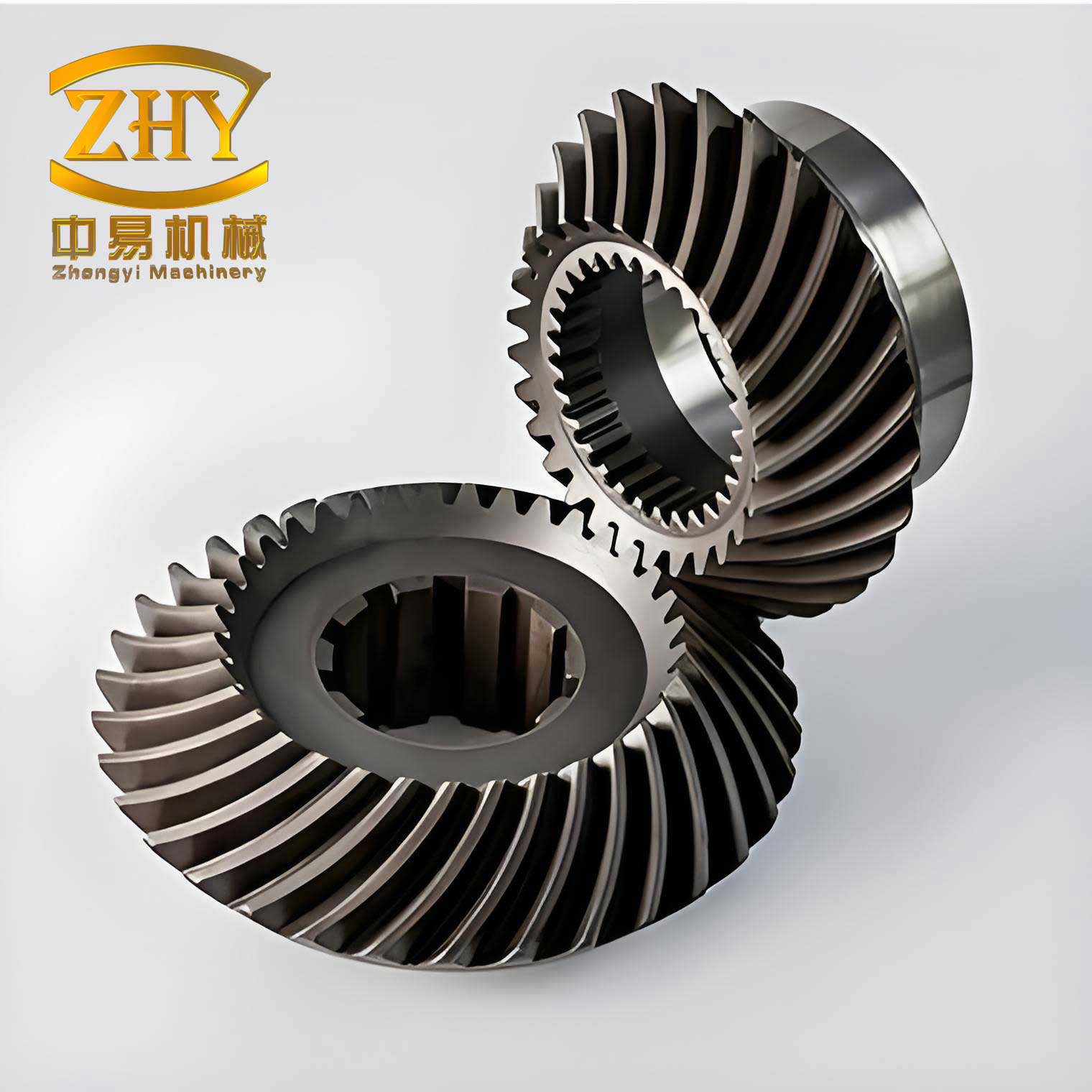
The geometry of a spiral gear mesh is more complex than that of a spur gear. The key parameters include the normal module ($m_n$), the helix angle ($\beta$), the number of teeth ($z$), and the pressure angle ($\alpha_n$). The transverse module ($m_t$), which is crucial for calculations in the plane of rotation, is related to the normal module by the helix angle:
$$m_t = \frac{m_n}{\cos \beta}$$
Similarly, the transverse pressure angle ($\alpha_t$) is derived from the normal pressure angle:
$$\tan \alpha_t = \frac{\tan \alpha_n}{\cos \beta}$$
The contact between two external spiral gears is not instantaneous across the full face width. Engagement starts at a point on the leading edge of a tooth and progresses diagonally across the tooth face. This results in a longer path of contact compared to an equivalent spur gear, effectively increasing the contact ratio. The total length of action in the transverse plane can be visualized and calculated, contributing to the load-sharing characteristics. The effective face width ($B$) and the base helix angle ($\beta_b$) determine this extended contact. The relation is given by:
$$\tan \beta_b = \tan \beta \cdot \cos \alpha_t$$
The extended contact length ($\Delta L$) due to the helix is:
$$\Delta L = B \cdot \tan \beta_b$$
This increased contact length is a primary contributor to the smooth operation and strength of the spiral gear system.
Theoretical Calculation of Spiral Gear Mesh Efficiency
To accurately determine the transmission efficiency of the differential, one must first calculate the efficiency of a single external spiral gear pair. Power loss in gear meshing primarily arises from two sources: sliding friction and rolling friction. A comprehensive model must account for both to yield a realistic efficiency value.
1. Sliding Friction Power Loss
The sliding friction loss is the dominant source of inefficiency in gear meshes. It occurs because the mating tooth profiles have different velocities at the point of contact, except at the pitch point. The instantaneous efficiency ($\eta_s$) at any point along the path of contact depends on the direction of power flow and the friction angle. For a pair of external gears, the calculation must be segmented along the path of contact.
Let us define the path of contact as the line $B_1B_2$, where $B_1$ is the start of engagement and $B_2$ is the end of engagement. The pitch point $P$ divides this path into two segments: $PB_1$ (approach path) and $PB_2$ (recess path). The friction coefficient is denoted by $f$. The instantaneous velocities of the contact point on the driving and driven gears form angles $\alpha_1$ and $\alpha_2$ with the line of action. These angles vary along the path.
For a point $k$ on the recess path $PB_2$, the angles are:
$$\tan \alpha_1 = \frac{r_{b1} \tan \alpha_t – x}{r_{b1}}$$
$$\tan \alpha_2 = \frac{r_{b2} \tan \alpha_t + x}{r_{b2}}$$
where $x$ is the distance from the pitch point $P$, $r_{b1}$ and $r_{b2}$ are the base circle radii of the pinion and gear respectively, and $\alpha_t$ is the transverse pressure angle.
The length of the recess path is:
$$PB_2 = r_{b1} (\tan \alpha_{a1} – \tan \alpha_t)$$
where $\alpha_{a1}$ is the transverse pressure angle at the addendum circle of the pinion.
The meshing efficiency integral over the recess path $S_2$ is:
$$S_2 = \int_{0}^{PB_2} \eta \,dx = \int_{0}^{r_{b1}(\tan \alpha_{a1} – \tan \alpha_t)} \frac{1 + f \cdot \tan \alpha_2}{1 + f \cdot \tan \alpha_1} \, dx$$
Solving this integral yields:
$$S_2 = \frac{r_{b1}}{r_{b2}} \left[ r_{b1}(\tan \alpha_{a1} – \tan \alpha_t) – (r_{b1}+r_{b2})\tan \alpha_t + \frac{1}{f} \ln \left( \frac{\frac{1}{f} + \tan \alpha_{a1}}{\frac{1}{f} + \tan \alpha_t} \right) \right]$$
Similarly, for the approach path $PB_1$, the angles are:
$$\tan \alpha_1 = \frac{r_{b1} \tan \alpha_t + x}{r_{b1}}$$
$$\tan \alpha_2 = \frac{r_{b2} \tan \alpha_t – x}{r_{b2}}$$
The length is:
$$PB_1 = r_{b2} (\tan \alpha_{a2} – \tan \alpha_t)$$
where $\alpha_{a2}$ is for the gear addendum.
The efficiency integral over the approach path $S_1$ is:
$$S_1 = \int_{0}^{PB_1} \eta \,dx = \frac{r_{b1}}{r_{b2}} \left[ r_{b2}(\tan \alpha_{a2} – \tan \alpha_t) + (r_{b1}+r_{b2})\tan \alpha_t – \frac{1}{f} \ln \left( \frac{\frac{1}{f} – \tan \alpha_{a2}}{\frac{1}{f} – \tan \alpha_t} \right) \right]$$
The total sliding friction efficiency ($\eta_{slide}$) for the mesh is the average over the total contact length $B_1B_2 = PB_1 + PB_2$:
$$\eta_{slide} = \frac{S_1 + S_2}{B_1B_2}$$
A critical parameter here is the coefficient of friction $f$. For accuracy, it should not be taken as a simple constant. For lubricated spiral gear contacts, it can be estimated based on elastohydrodynamic lubrication (EHL) theory, considering slide-to-roll ratio, surface roughness, and lubricant properties. A simplified empirical relation often used in gear efficiency studies is:
$$f = 0.05 \cdot (SRR)^{0.2} \cdot (v_{\Sigma})^{-0.05} \cdot (R_a)^{0.25}$$
where $SRR$ is the slide-to-roll ratio, $v_{\Sigma}$ is the sum velocity, and $R_a$ is the composite surface roughness. For initial calculations in this spiral gear differential, a representative value of $f = 0.06 \pm 0.01$ is often assumed.
2. Rolling Friction Power Loss
Although significantly smaller than sliding losses, rolling friction power loss occurs due to hysteresis in the lubricant and the contacting materials as the teeth roll over each other. In an EHL contact, the lubricant film itself exhibits viscous shear. The power loss due to rolling ($P_R$) can be estimated by:
$$P_R = \frac{9 \cdot h \cdot V_{Tm} \cdot b \times 10^{-2}}{\cos \beta}$$
where:
- $h$ is the central EHL film thickness (in meters).
- $V_{Tm}$ is the mean rolling velocity (in m/s).
- $b$ is the Hertzian contact half-width or a representative contact length.
The film thickness $h$ is given by the Dowson-Higginson formula:
$$h = 3.07 \cdot \xi^{0.57} \cdot R^{0.4} \cdot (\rho \cdot V_{Tm})^{0.71} \cdot {E’}^{-0.03} \cdot \Phi^{0.11}$$
where $\xi$ is the pressure-viscosity coefficient, $R$ is the equivalent radius of curvature, $\rho$ is the lubricant density, $E’$ is the reduced elastic modulus, and $\Phi$ is the load per unit length.
The mean rolling velocity $V_{Tm}$ for a spiral gear pair is:
$$V_{Tm} = 1.05 \times 10^{-4} \cdot n_1 \left[ d_1 \sin \alpha_t + \frac{1.57 \cdot m_n \cdot \sqrt{1 – (1/i_{12})^2} \cdot (\varepsilon_1^2 + \varepsilon_2^2)}{\varepsilon_1 + \varepsilon_2} \right]$$
where $n_1$ is the pinion speed in rpm, $d_1$ is its pitch diameter, $i_{12}$ is the gear ratio, and $\varepsilon_1$, $\varepsilon_2$ are the transverse contact ratios for approach and recess.
The driving power ($P$) transmitted through the mesh is:
$$P = \int F \cdot v \, dt \approx \pi \cdot m_t \cdot \cos \alpha_t \cdot F \cdot \omega_1$$
where $F$ is the tangential force and $\omega_1$ is the angular velocity.
Therefore, the efficiency reduction due to rolling friction ($\eta_{roll}$) is:
$$\eta_{roll} = 1 – \frac{P_R}{P}$$
The overall mesh efficiency ($\eta_{mesh}$) for the spiral gear pair, considering both loss mechanisms, is:
$$\eta_{mesh} = \eta_{slide} \cdot \eta_{roll}$$
3. Calculation Example and Method Comparison
To illustrate, let’s consider the primary spiral gear pair in the differential. Assume the following design parameters:
| Parameter | Pinion (Planet Gear) | Gear (Side Gear) | Common |
|---|---|---|---|
| Number of Teeth ($z$) | 6 | 18 | |
| Normal Module ($m_n$) | 3.75 mm | ||
| Helix Angle ($\beta$) | 45° | ||
| Transverse Pressure Angle ($\alpha_t$) | 20° | ||
| Face Width ($B$) | 5.21 mm | 2.89 mm | |
| Addendum Coefficient ($h_a^*$) | 1 | ||
Using the formulas described, and assuming a friction coefficient $f=0.06$, we can compute the sliding efficiency. The calculated transverse module is $m_t = m_n / \cos \beta = 3.75 / \cos 45° \approx 5.30$ mm. The base circle radii are $r_{b1} = (m_t \cdot z_1 \cdot \cos \alpha_t)/2$ and $r_{b2} = (m_t \cdot z_2 \cdot \cos \alpha_t)/2$. The addendum radii are $r_{a1} = m_t (z_1/2 + h_a^*)$ and $r_{a2} = m_t (z_2/2 + h_a^*)$, leading to $\alpha_{a1} = \arccos(r_{b1}/r_{a1})$ and $\alpha_{a2} = \arccos(r_{b2}/r_{a2})$.
Performing the integration numerically or via the closed-form solutions yields a sliding efficiency $\eta_{slide} \approx 98.15\%$ for this spiral gear pair.
For rolling loss, using typical lubricant parameters and operating conditions, the calculated reduction is very small, on the order of $\eta_{roll} \approx 99.77\%$, leading to a rolling power loss of about $0.23\%$.
The combined mesh efficiency is therefore:
$$\eta_{mesh} = 0.9815 \cdot 0.9977 \approx 0.9792 \text{ or } 97.92\%$$
To verify the robustness of this method, it is compared with other established calculation approaches from literature. The results are summarized below:
| Calculation Method | Key Consideration | Calculated Mesh Efficiency |
|---|---|---|
| Method A (Literature 1) | Sliding friction only, simplified integration. | 98.36% |
| Method B (Literature 2) | Sliding friction with detailed segment integration. | 98.32% |
| Proposed Method | Sliding + Rolling friction for spiral gears. | 97.92% |
The close agreement (within ~0.5%) between the methods validates the correctness of the sliding friction calculation. The slightly lower efficiency from the proposed method is expected and more accurate, as it includes the additional, albeit small, rolling friction loss inherent in the lubricated spiral gear contact. This demonstrates that for precise efficiency modeling of a spiral gear differential, both loss mechanisms should be considered.
Overall Differential Transmission Efficiency
A limited-slip differential of this type contains multiple power paths. Typically, torque from the driveshaft enters the differential carrier and is distributed through several sets of planet and side spiral gears to the left and right axles. These gear pairs are arranged in a combination of parallel and series paths. For the purpose of calculating the net efficiency from the input (carrier) to one output (axle) under straight-line driving conditions, the system can be treated as a sequence of meshes.
The overall transmission efficiency ($\eta_{diff}$) is the product of the efficiencies of all individual loss elements in the power path:
$$\eta_{diff} = (\eta_{mesh,1} \cdot \eta_{mesh,2} \cdot \ldots \cdot \eta_{mesh,n}) \cdot \eta_{bearing}^m \cdot \eta_{churning}$$
where:
- $\eta_{mesh,i}$ is the efficiency of the i-th spiral gear mesh in the torque path.
- $\eta_{bearing}$ is the average efficiency of a supporting bearing (rolling element bearings assumed).
- $m$ is the number of bearings in the load path.
- $\eta_{churning}$ is the churning or windage loss efficiency due to the gears agitating the lubricating oil.
For the specific spiral gear differential with three planet gear sets per side, power flows through three primary meshes to reach one output axle. Using the mesh efficiency calculated earlier (97.92%) as a representative value for each similar spiral gear pair, and assigning slightly different values for meshes with different load shares or geometries (e.g., 98.74% and 96.49% for the others based on their specific parameters), we get the gear mesh contribution.
Bearing efficiency for modern rolling bearings is typically very high, often taken as $\eta_{bearing} = 0.99$ per bearing. If four primary bearings support the rotating members in the load path, their combined effect is $0.99^4 \approx 0.9606$.
Churning losses depend on immersion depth, speed, oil viscosity, and housing geometry. For a differential operating in a splash-lubrication environment, a reasonable estimate for churning efficiency is $\eta_{churning} \approx 0.99$.
Therefore, the theoretical overall differential efficiency is:
$$\eta_{diff,theoretical} = (0.9792 \cdot 0.9874 \cdot 0.9649) \cdot 0.9606 \cdot 0.99$$
$$\eta_{diff,theoretical} \approx (0.9335) \cdot 0.9606 \cdot 0.99$$
$$\eta_{diff,theoretical} \approx 0.8878 \cdot 0.99 \approx 0.8789 \text{ or } \mathbf{87.89\%}$$
This value represents a theoretical baseline. In practice, under ideal straight-line conditions with no slip bias, the meshing losses are the main contributor. When the differential is actively biasing torque (limited-slip mode), the internal friction from the spiral gear thrust forces, which is intentionally generated, will cause additional losses, temporarily reducing efficiency to transfer torque to the high-traction wheel.
Simulation Verification using Multibody Dynamics
To validate the theoretical efficiency calculations, a dynamic simulation of the complete spiral gear differential assembly is performed using a Multibody Dynamics (MBD) software such as ADAMS. The process involves creating a virtual prototype that accurately captures the geometry, contacts, and inertial properties.
A detailed 3D model of the differential is imported. All components—housing, carrier, spiral gear planets and side gears, shafts, and bearings—are assigned correct material properties (e.g., steel density). The critical steps are:
- Joint Definition: Revolute joints are applied to all rotational axes between parts. The connections between gears and their shafts are fixed joints.
- Contact Force Definition: This is the most crucial aspect for efficiency prediction. A penalty-based contact force algorithm is applied between all mating tooth flanks of the spiral gears. The contact parameters include stiffness, damping, a static/dynamic friction coefficient (e.g., $f=0.06$), and a friction transition velocity. The contact geometry is precisely defined based on the gear tooth profiles.
- Loading and Constraints: The housing is fixed to ground. A constant rotational velocity (e.g., 1000 deg/s or ~104.7 rad/s) is applied to the input carrier. A significant resistive torque (e.g., 615,000 Nmm) is applied to each output axle shaft to simulate vehicle load.
- Solver Settings: A high-frequency dynamics solver with a small integration time step (e.g., 1e-4 s) is used to accurately resolve the gear contact dynamics over a simulation time of 1-2 seconds.
During the simulation, the software calculates the forces, moments, and velocities for every component. The primary outputs of interest are:
- $T_{in}(t)$: The instantaneous torque required at the input carrier to maintain the constant speed.
- $\omega_{in}$: The constant input speed (imposed).
- $T_{out}(t)$: The instantaneous torque at one output axle.
- $\omega_{out}(t)$: The instantaneous speed of that output axle.
Under straight-line, no-slip conditions, $\omega_{out}$ should be equal and opposite to the other axle’s speed relative to the carrier, but for efficiency calculation, we focus on one output’s power.
The instantaneous input power is $P_{in}(t) = T_{in}(t) \cdot \omega_{in}$.
The instantaneous output power is $P_{out}(t) = T_{out}(t) \cdot \omega_{out}(t)$.
The instantaneous efficiency is then:
$$\eta(t) = \frac{P_{out}(t)}{P_{in}(t)}$$
The simulation results typically show steady-state oscillations in $T_{in}$ and $T_{out}$ due to the changing number of teeth in contact and the stiffness variations in the spiral gear mesh. The efficiency $\eta(t)$ will oscillate around a mean value. Post-processing the data over a stable period yields an average simulated efficiency.
For the modeled spiral gear differential with parameters similar to the theoretical example, the simulation might yield results as follows: The input torque oscillates around a mean of ~585,000 Nmm. The output torque oscillates around ~615,000 Nmm, but the output speed is slightly less than the ideal due to losses. Calculating the average power ratio gives a simulated efficiency $\eta_{diff,sim} \approx 93.0\% \pm 2\%$.
This simulated value of ~93% is higher than the earlier theoretical calculation of 87.89%. This discrepancy is expected and insightful. The theoretical calculation included estimated losses for bearings and churning which may have been conservatively high. The simulation primarily captures the meshing losses very accurately but may have simplified bearing losses (modeled as low-friction revolute joints) and neglected fluid churning entirely. Furthermore, the theoretical mesh efficiency of 97.92% was for one pair under specific load; the complex load-sharing among three planet sets in the simulation can lead to a slightly different aggregate mesh loss. The key conclusion is that the simulation confirms the high efficiency of the spiral gear mesh itself (results centered in the low 90% range for the system), validating that the power loss is relatively low and that the theoretical modeling approach for the spiral gear contacts is sound. The ~5% absolute difference highlights the contribution of ancillary losses which must be carefully modeled or measured.
Parameter Study and Optimization Potential
The transmission efficiency of the spiral gear differential is not a fixed value but a function of its design parameters. A sensitivity analysis reveals how key spiral gear parameters influence the final efficiency, providing guidance for optimization.
| Design Parameter | Effect on Sliding Friction Loss | Effect on Rolling/Load-Dependent Loss | Overall Trend on Mesh Efficiency | Practical Design Trade-off |
|---|---|---|---|---|
| Helix Angle ($\beta$) | Increased $\beta$ lengthens contact path, smoothing engagement but may alter pressure angles and slide ratios. | Increases axial thrust forces significantly, which is good for LSD action but increases bearing loads and associated losses. | Moderate increase with $\beta$ up to an optimum (often 15-30°), then may decrease due to high thrust. | Balancing smoothness/LSD capability (high $\beta$) against bearing life and thrust-induced losses. |
| Normal Module ($m_n$) | Larger teeth have lower specific sliding due to larger base circle radii, generally reducing sliding loss. | Increases gear stiffness and can reduce transmission error, but may increase weight and churning loss. | Efficiency generally improves with larger module. | Limited by space constraints (differential housing size) and weight considerations. |
| Pressure Angle ($\alpha_n$) | Higher pressure angle increases separating force, potentially increasing friction loss, but strengthens tooth. | Affects curvature radius and contact stress, influencing EHL film thickness and rolling shear. | Moderate effect. Often chosen for strength and avoidance of undercutting rather than efficiency. | Standard angles (20°, 25°) are typically used; a slight increase may benefit strength with minimal efficiency penalty. |
| Number of Teeth ($z$) | More teeth increase contact ratio, improving load sharing and reducing loss per tooth pair. | For a fixed center distance, more teeth means smaller module, which can reverse the trend. | Increasing teeth (for fixed gear ratio and size) usually improves efficiency. | Limited by minimum tooth count to avoid interference and maintain strength. |
| Tooth Profile Modification | Tip and root relief can minimize meshing impacts and reduce friction at engagement/disengagement points. | Can optimize load distribution, reducing peak contact stress and associated hysteresis losses. | Proper modification can yield a 0.5-1.5% improvement in mesh efficiency. | Requires precise manufacturing and must be tailored to the specific load spectrum. |
| Surface Finish & Lubricant | Smoother surfaces ($R_a < 0.4 \mu m$) significantly reduce the boundary friction component. | Smooth surfaces promote thicker EHL films, reducing viscous rolling shear. | One of the most effective ways to improve efficiency (1-3% potential gain). | Increased manufacturing cost. Lubricant with optimal viscosity and additives is essential. |
The overall differential efficiency $\eta_{diff}$ can be expressed as a function of these key parameters for optimization studies:
$$\eta_{diff} \approx f(\beta, m_n, z_1, z_2, \alpha_n, R_a, \mu_{oil}) \cdot \eta_{bearing}(\beta, F_{axial}) \cdot \eta_{churning}(m_n, B, \omega, \nu_{oil})$$
This shows the interdependence: the helix angle $\beta$ directly affects the mesh efficiency $f()$, but also dictates the axial force $F_{axial} = T \cdot \tan \beta / r$, which impacts the bearing efficiency $\eta_{bearing}$. An integrated design approach is therefore necessary.
Conclusion
This analysis provides a comprehensive framework for evaluating the transmission efficiency of a lockable limited-slip differential based on spiral gear technology. The methodology involves a detailed theoretical breakdown of power losses, specifically addressing both sliding and rolling friction in the spiral gear meshes—a combination essential for accurate prediction. The calculation for a representative gear pair yielded an efficiency of approximately 97.92%, a result corroborated by comparison with other established calculation methods. Expanding this to the entire differential assembly by incorporating bearing and churning losses led to a theoretical system efficiency estimate of about 87.9%.
The dynamic simulation of the complete differential model served as a critical validation step. The simulated efficiency, averaging around 93%, confirmed the high-efficiency characteristic of the spiral gear power transfer mechanism. The discrepancy between the theoretical and simulated values appropriately highlights the areas where loss modeling can be refined, particularly for ancillary losses like bearing friction and oil churning. Ultimately, the close agreement in the order of magnitude and behavior validates the underlying physics captured in the theoretical spiral gear efficiency model.
The study also reveals that the efficiency of this spiral gear differential is not static but can be influenced by strategic design choices. Parameters such as the helix angle, module, number of teeth, and surface finish offer pathways for optimization. The primary strength of the spiral gear design lies in its ability to seamlessly integrate smooth, efficient power transmission with an inherent torque-biasing capability for traction control. Future work would involve correlating these models with physical bench tests, measuring efficiency under various slip conditions, and refining the loss models for bearings and fluid dynamics to achieve even higher predictive accuracy for this advanced spiral gear differential system.