
The study of elastohydrodynamic lubrication (EHL) represents a cornerstone in the design and analysis of highly loaded machine elements, particularly gears. The classical EHL theory, which matured in the 1960s, elegantly combines the Reynolds equation of fluid film lubrication with the Hertzian theory of elastic contact. For spur gears operating under high speed and heavy load conditions, the lubrication regime within the tooth contact directly governs performance metrics such as efficiency, wear, and fatigue life. The instantaneous load, curvature, and surface velocities vary significantly throughout the meshing cycle of spur gears, making the numerical analysis of film thickness and pressure a challenging task. This article presents a comprehensive numerical study of isothermal line contact EHL applicable to involute spur gears, employing the multigrid method for enhanced stability and efficiency. Furthermore, it extends the analysis to compute the sliding friction coefficient over an entire meshing period, investigating its dependence on operational parameters like rotational speed.
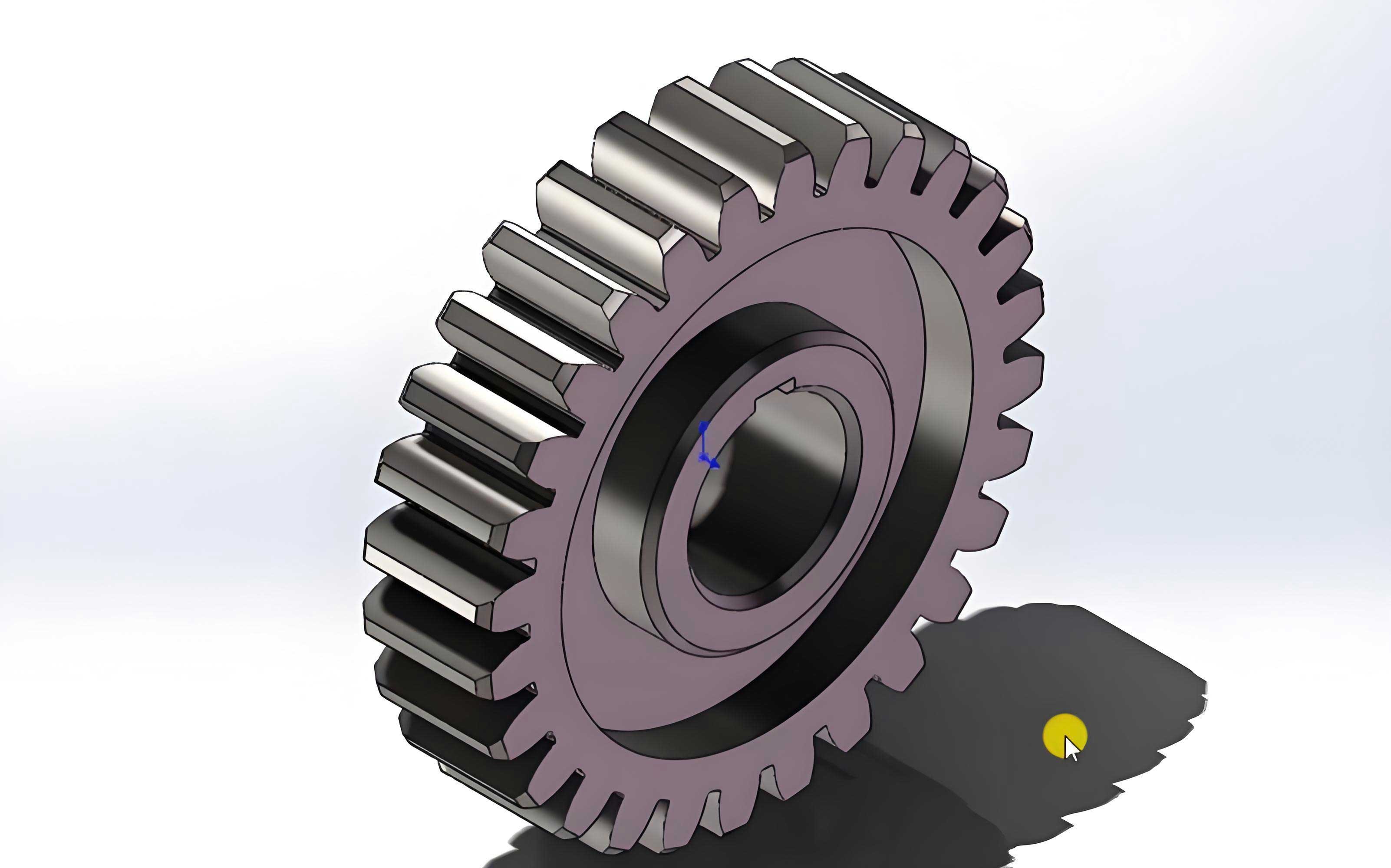
The contact between two teeth in a pair of meshing involute spur gears can be accurately modeled as the contact between two equivalent elastic cylinders. According to Hertzian theory, under a normal load \(w\), the cylinders deform, creating a narrow rectangular contact zone of half-width \(b\), rather than a theoretical line contact. The pressure distribution across this zone, in the dry contact scenario, is semi-elliptical. The geometry of involute spur gears dictates that the radii of curvature of the contacting teeth change continuously as the contact point moves from the root to the tip along the path of action. This results in a time-varying equivalent radius of curvature \(R\) and a varying entrainment velocity \(u_s\), both critical inputs for EHL analysis. The load is also shared between one or two pairs of teeth depending on the contact ratio, leading to a piecewise function for the instantaneous load per unit face width.
Governing Equations for Isothermal Line Contact EHL
The foundation of the analysis is the one-dimensional Reynolds equation, which for a steady-state, isothermal line contact with considering film thickness variation, is given by:
$$\frac{d}{dx}\left( \frac{\rho h^3}{\eta} \frac{dp}{dx} \right) = 12 u_s \frac{d(\rho h)}{dx}$$
where \(p\) is the film pressure, \(h\) is the film thickness, \(\eta\) is the dynamic viscosity, \(\rho\) is the fluid density, \(x\) is the coordinate along the direction of motion, and \(u_s = (u_1 + u_2)/2\) is the entrainment or rolling velocity, with \(u_1\) and \(u_2\) being the surface velocities of the two contacting bodies (gear teeth).
To facilitate numerical solution and generalize the results, the equation is non-dimensionalized. Common dimensionless groups are introduced:
$$X = \frac{x}{b}, \quad P = \frac{p}{p_h}, \quad H = \frac{hR}{b^2}, \quad \bar{\eta} = \frac{\eta}{\eta_0}, \quad \bar{\rho} = \frac{\rho}{\rho_0}$$
where \(b\) is the Hertzian half-width, \(p_h\) is the maximum Hertzian pressure, \(R\) is the effective radius of curvature, and \(\eta_0\) and \(\rho_0\) are the ambient viscosity and density, respectively. The dimensionless Reynolds equation becomes:
$$\frac{d}{dX}\left( \varepsilon \frac{dP}{dX} \right) – \frac{d(\bar{\rho} H)}{dX} = 0$$
where \(\varepsilon = \frac{\bar{\rho} H^3}{\bar{\eta} \lambda}\), and \(\lambda = \frac{12 \eta_0 u_s R^2}{b^3 p_h}\) is a dimensionless speed parameter. The boundary conditions are \(P(X_{in}) = 0\) at the inlet and the Reynolds exit condition \(P(X_{out}) = \frac{dP}{dX}(X_{out}) = 0\) at the outlet.
The film thickness equation accounts for the geometric gap and the elastic deformation of the surfaces caused by the pressure distribution:
$$h(x) = h_0 + \frac{x^2}{2R} – \frac{2}{\pi E’} \int_{x_{in}}^{x_{out}} p(s) \ln|x-s| ds$$
In dimensionless form, this is expressed as:
$$H(X) = H_0 + \frac{X^2}{2} – \frac{1}{2\pi} \int_{X_{in}}^{X_{out}} P(S) \ln|X-S| dS$$
Here, \(h_0\) (or \(H_0\)) is a central offset, and \(E’\) is the effective elastic modulus, defined for two bodies with Young’s moduli \(E_1, E_2\) and Poisson’s ratios \(\nu_1, \nu_2\) as:
$$\frac{1}{E’} = \frac{1}{2} \left( \frac{1-\nu_1^2}{E_1} + \frac{1-\nu_2^2}{E_2} \right)$$
The pressure dependence of lubricant properties is crucial in the high-pressure EHL regime. The viscosity-pressure relationship is often described by the Roelands equation:
$$\eta(p) = \eta_0 \exp \left\{ (\ln(\eta_0) + 9.67) \left[ (1 + 5.1 \times 10^{-9} p)^Z – 1 \right] \right\}$$
where \(Z\) is the pressure-viscosity index. The density-pressure relationship follows the Dowson-Higginson formula:
$$\rho(p) = \rho_0 \left( 1 + \frac{0.6 \times 10^{-9} p}{1 + 1.7 \times 10^{-9} p} \right)$$
Finally, the solution must satisfy the force balance equation, ensuring the integrated pressure supports the applied load \(w\) per unit length:
$$\int_{x_{in}}^{x_{out}} p(x) dx = w$$
In its dimensionless form:
$$\int_{X_{in}}^{X_{out}} P(X) dX = \frac{\pi}{2}$$
Numerical Solution via the Multigrid Method
The system of coupled, non-linear integral-differential equations (Reynolds, film thickness, force balance) presents a significant computational challenge. The Full Approximation Scheme (FAS) multigrid method is exceptionally effective for solving such EHL problems. The core idea is to use a hierarchy of grids with different spacings to efficiently eliminate error components of all frequencies.
A set of grids \(G^k\) (\(k=1,2,…,m\)) is defined, where \(G^1\) is the finest grid and \(G^m\) the coarsest. The non-linear discrete problem on the finest grid \(G^1\) is denoted as:
$$L^1(P^1) = F^1$$
For the coarser grids (\(k > 1\)), the equation to be solved is not the original discrete equation, but the defect equation. This equation is designed to correct the current approximation. If \(\tilde{P}^k\) is an approximate solution on grid \(G^k\), and \(I_k^{k-1}\) is an interpolation operator from grid \(G^{k-1}\) to \(G^k\), the defect equation on grid \(G^k\) is:
$$L^k(P^k) = L^k(I_k^{k-1} \tilde{P}^{k-1}) + \tau_k^{k-1}$$
where \(\tau_k^{k-1} = F^k – I_k^{k-1} F^{k-1}\) is the defect or fine-to-coarse residual transfer. The right-hand side \(F^k\) typically contains the term \(-\frac{d(\bar{\rho} H)}{dX}\). The discretized form of the defect equation for the Reynolds equation at an interior node \(i\) on grid \(k\) is:
$$\frac{1}{\Delta X^k} \left[ \varepsilon_{i-1/2}^k \frac{P_{i-1}^k – P_i^k}{\Delta X^k} – \varepsilon_{i+1/2}^k \frac{P_i^k – P_{i+1}^k}{\Delta X^k} \right] – \frac{(\bar{\rho} H)_{i}^k – (\bar{\rho} H)_{i-1}^k}{\Delta X^k} = (F^k)_i$$
where \(\varepsilon_{i\pm1/2} = (\varepsilon_i + \varepsilon_{i\pm1})/2\). Similarly, the force balance defect equation on grid \(k\) is:
$$\Delta X^k \sum_{j=1}^{n_k-1} \frac{P_j^k + P_{j+1}^k}{2} = \frac{\pi}{2} + g^k$$
The constant \(g^k\) is the transferred defect from the finer grid’s force balance. This equation is used to update the rigid film thickness \(H_0^k\) iteratively. If the integrated pressure is greater than the required load, the film is too thin, so \(H_0\) must be increased, and vice versa. The update scheme is:
$$(H_0^k)^{new} = (H_0^k)^{old} + \omega_2 \left[ \frac{\pi}{2} – \Delta X^k \sum_{j=1}^{n_k-1} \frac{P_j^k + P_{j+1}^k}{2} + g^k \right]$$
where \(\omega_2\) is an under-relaxation factor (e.g., 0.02).
The solution process follows a W-cycle for robust convergence. On each grid level, a few relaxation sweeps (e.g., Gauss-Seidel) are performed to smooth the high-frequency errors. The residuals are then restricted to the next coarser grid to correct the low-frequency errors. The corrected solution is interpolated back to finer grids. This cycle repeats until convergence on the finest grid is achieved. This method is applied to analyze the contact in spur gears at discrete points along the path of action.
| Parameter | Symbol | Value / Range | Unit |
|---|---|---|---|
| Number of Teeth (Drive) | \(z_1\) | 43 | – |
| Number of Teeth (Driven) | \(z_2\) | 60 | – |
| Module | \(m_n\) | 3.1 | mm |
| Pressure Angle | \(\alpha\) | 20 | ° |
| Face Width | \(B\) | 60 | mm |
| Input Power | \(P_{in}\) | 212.83 | kW |
| Input Speed | \(n\) | 1000 – 1500 | rpm |
| Effective Elastic Modulus | \(E’\) | 2.26e11 | Pa |
| Ambient Viscosity | \(\eta_0\) | 0.08 | Pa·s |
| Ambient Density | \(\rho_0\) | 870 | kg/m³ |
| Roelands Exponent | \(Z\) | 0.6 (example) | – |
Friction Coefficient in EHL Contacts
Under fully developed elastohydrodynamic lubrication in spur gears, the total friction force arises from both sliding and rolling components. The sliding friction force per unit width, \(F_t\), can be derived by integrating the shear stress across the film. For a Newtonian fluid, it is proportional to the velocity difference and inversely proportional to film thickness. However, under high shear stress, non-Newtonian behavior (e.g., Eyring fluid) becomes important. The shear stress \(\tau\) for an Eyring fluid with characteristic shear stress \(\tau_0\) is related to the shear rate \(\dot{\gamma}\) by:
$$\tau = \tau_0 \sinh^{-1}\left( \frac{\eta \dot{\gamma}}{\tau_0} \right)$$
The effective viscosity is then \(\eta^* = \tau / \dot{\gamma} = \eta \frac{\tau_0 / \tau}{\sinh^{-1}(\eta \dot{\gamma} / \tau_0)}\). Assuming a linear velocity profile across the film, the shear rate is \(\dot{\gamma} = (u_2 – u_1)/h + (h/2\eta)(dp/dx)\). The shear stress at a point in the contact is a function of this shear rate and the pressure gradient. For contacts in spur gears where the slide-to-roll ratio is significant, the contribution from pure rolling friction is often negligible compared to sliding friction. Therefore, the sliding friction force can be approximated by integrating the shear stress due to sliding across the contact:
$$F_t \approx \int_{x_{in}}^{x_{out}} \eta^* \frac{(u_2 – u_1)}{h} dx$$
The instantaneous coefficient of friction \(\mu\) is then defined as the ratio of this friction force to the total normal load \(W\) acting on the contact at that instant:
$$\mu = \frac{F_t}{W}$$
where \(W = w \times B\) (load per unit length times face width). For a meshing cycle of spur gears, both \(u_1\), \(u_2\), \(h\), \(w\), and consequently \(\mu\), vary with the contact position.
Case Study: Results and Discussion
The analysis is performed for a specific gear pair. The load distribution across the path of action is first calculated based on the contact ratio, yielding a piecewise function for the load sharing between one and two pairs of teeth. This load distribution is a critical input for the sequential EHL calculations at discrete meshing positions. The following presents key results for different input speeds (1000, 1200, 1400, 1500 rpm).
Instantaneous Pressure and Film Thickness: At any given instant in the meshing cycle, the solution of the EHL system yields characteristic pressure and film thickness profiles. The pressure profile closely follows the Hertzian ellipse in the central region but exhibits a sharp secondary pressure spike near the outlet. The film thickness profile is nearly parallel in the central region but constricts at the outlet, forming a characteristic “neck.” The central and minimum film thickness values increase significantly with increasing rotational speed, as higher entrainment velocity \(u_s\) pumps more lubricant into the contact. The maximum pressure and the secondary pressure spike show a relatively mild increase with speed.
| Speed (rpm) | Entrainment Velocity \(u_s\) (m/s) | Dim. Load Parameter | Central Film Thickness \(h_c\) (µm) | Min. Film Thickness \(h_{min}\) (µm) | Max. Pressure \(p_{max}\) (GPa) |
|---|---|---|---|---|---|
| 1000 | 3.5 | 1.326e-4 | 0.85 | 0.75 | 0.92 |
| 1200 | 4.2 | 1.326e-4 | 0.98 | 0.82 | 0.93 |
| 1400 | 4.9 | 1.326e-4 | 1.10 | 0.88 | 0.94 |
| 1500 | 5.25 | 1.326e-4 | 1.16 | 0.92 | 0.95 |
Minimum Film Thickness Over Meshing Cycle: The minimum film thickness \(h_{min}\) is tracked throughout the path of action. Key observations are: In the double-tooth contact regions near the beginning and end of the meshing cycle, the load per tooth is lower, but the entrainment velocity is also relatively low, resulting in a modest film thickness. As the contact point moves towards the pitch point within a double-tooth zone, the entrainment velocity increases, causing \(h_{min}\) to rise gradually. At the transition from double-to-single tooth contact, the load on the single tooth suddenly doubles. This causes a sharp, transient decrease in \(h_{min}\) due to the increased Hertzian pressure squeezing the film. Within the single-tooth contact region, the load is constant, but the entrainment velocity continues to increase, leading to a steady recovery and increase in \(h_{min}\). The transition from single-to-double tooth contact sees a load relief and a corresponding jump in film thickness. Overall, \(h_{min}\) increases with the rotational speed at all meshing positions.
Friction Coefficient Over Meshing Cycle: The friction coefficient \(\mu\) shows a distinct and repeatable pattern over the meshing cycle of the spur gears. In the double-tooth contact regions, the friction coefficient tends to increase with the absolute distance from the pitch point. This is primarily because the sliding velocity \(|u_2 – u_1|\) increases linearly with this distance, while the load and film thickness changes are less dramatic. At the pitch point itself, pure rolling occurs (\(u_1 = u_2\)), leading to a theoretical sliding friction coefficient of zero (or a very small value from numerical approximation). In the single-tooth contact region, the friction coefficient increases nearly linearly from zero at the pitch point to a maximum at the boundaries of this zone. The single-to-double tooth transition points are critical: the sudden load increase causes a significant drop in film thickness. The consequent rise in lubricant effective viscosity (due to the higher pressure) and the maintained high sliding velocity lead to a sharp peak in the friction coefficient at these transition points. The numerical value of the friction coefficient is highly sensitive to speed. Higher speeds generate thicker films, which reduce the effective shear rate and the shear stress for a given slide-to-roll ratio, generally leading to lower friction coefficients across the meshing cycle, though the overall shape of the friction curve remains consistent.
Conclusions
This investigation demonstrates a robust numerical framework for analyzing the transient elastohydrodynamic lubrication in involute spur gears. The application of the multigrid Full Approximation Scheme provides stable and efficient solutions for the highly non-linear EHL equations at multiple points along the gear meshing path. The results clearly illustrate the complex interplay between time-varying load, geometry, and kinematics in determining the lubricant film thickness and pressure. The film thickness is predominantly governed by the entrainment velocity and is significantly enhanced by increasing rotational speed, a key design consideration for preventing metal-to-metal contact. The friction coefficient, derived from the EHL film conditions, exhibits a characteristic profile with minima at the pitch point and maxima near the engagement/disengagement regions, where adverse conditions of high sliding and sudden loading coincide. Understanding this profile is essential for accurately predicting the mechanical efficiency and thermal loading in gear drives. The methodology and findings presented form a solid basis for the advanced tribological design and analysis of spur gears and similar machine elements operating in the elastohydrodynamic regime.