
The quest for high-precision motion control in applications ranging from space robotics to advanced medical devices consistently drives the need for superior transmission mechanisms. Among these, the strain wave gear, also known as a harmonic drive, stands out due to its unique operating principle and compelling advantages. Its compact design, high torque capacity, near-zero backlash, and substantial single-stage reduction ratios make it an indispensable component in precision servo systems. However, the very flexibility that enables its operation also introduces complex dynamical behaviors that challenge conventional control strategies. This article delves into the intricate control problem of strain wave gear systems, presenting a robust solution to manage the multiple, coupled disturbances inherent in their operation.
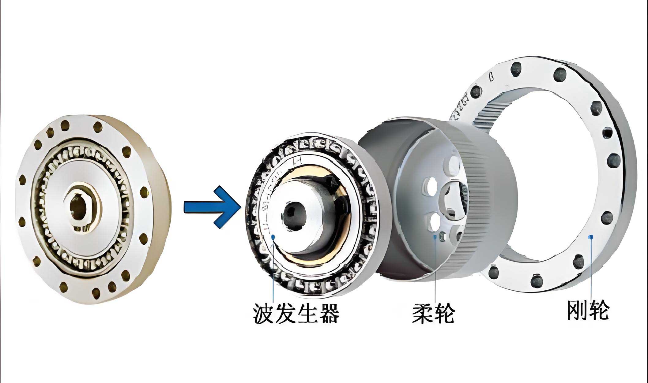
At its core, a strain wave gear system comprises three primary components: a rigid Circular Spline (CS), a flexible Flexspline (FS), and an elliptical Wave Generator (WG). The WG deforms the FS, causing its external teeth to engage with the internal teeth of the CS at two opposing points. As the WG rotates, the engagement point travels, resulting in a relative motion between the FS and CS. The high reduction ratio is achieved because the FS has slightly fewer teeth than the CS. The fundamental kinematic relationship in an ideal system is given by:
$$
\theta_{WG} = (N + 1)\theta_{CS} – N\theta_{FS}
$$
where $\theta_{WG}$, $\theta_{CS}$, and $\theta_{FS}$ are the angular positions of the WG, CS, and FS, respectively, and $N$ is the gear reduction ratio. In a typical configuration where the CS is fixed, the relationship simplifies, showing that the FS output rotates in the opposite direction to the WG input at a speed reduced by a factor of $N$.
While elegant in principle, the real-world dynamics of a strain wave gear are far from this simple proportional relationship. The system is plagued by multiple, intertwined sources of disturbance that severely degrade positioning accuracy if not explicitly addressed. Treating the strain wave gear as a simple gain is insufficient for precision applications. The primary disturbances can be categorized as follows:
- Kinematic Error ($\Delta \theta_p$): A periodic error arising from manufacturing tolerances and assembly imperfections, best modeled by a Fourier series expansion.
- Flexible Stiffness ($T$): The nonlinear torsional stiffness resulting from the elastic deformation of the FS and the WG bearing. It is often represented by a polynomial function of the torsional angle.
- Friction ($\tau_f$): Resistive torques from gear meshing and bearing contacts, which can be modeled statically (e.g., Stribeck) or dynamically (e.g., LuGre model).
- Hysteresis ($q$): A rate-dependent, memory-based nonlinearity causing a phase lag and amplitude dependence between input and output, arising from the coupling of friction and flexibility. It is frequently modeled using structures like the Bouc-Wen model.
These disturbances are not merely additive; they interact with each other and with the system states in complex ways, acting through multiple channels (both motor and load side). A comprehensive dynamic model considering these effects, derived from the Lagrange equation, is complex. For control design and simulation, a simplified yet representative model is essential. A common simplified state-space representation of the strain wave gear system is given by:
$$
\begin{aligned}
\dot{x}_1 &= x_2, \\
\dot{x}_2 &= \frac{1}{J_l} f_0 – \frac{B_l}{J_l} x_2 – \frac{1}{J_l} x_5, \\
\dot{x}_3 &= x_4, \\
\dot{x}_4 &= \frac{1}{J_m N} f_0 – \frac{\tau_f}{J_m} + \frac{1}{J_m N} x_5 + \frac{1}{J_m}(u + d), \\
\dot{x}_5 &= -\alpha |q_0| x_5 + A q_0,
\end{aligned}
$$
where the state vector is $\mathbf{x} = [\theta_{FS}, \dot{\theta}_{FS}, \theta_{WG}, \dot{\theta}_{WG}, q]^T$, $u = \tau_m$ is the motor control torque, and $d$ is an external disturbance. The terms $f_0$ and $q_0$ encapsulate the nonlinear stiffness and the internal hysteresis state derivative, respectively:
$$
\begin{aligned}
f_0 &= T\left(x_1 – \frac{x_3}{N} + b_2 \sin(2x_3)\right), \\
q_0 &= x_2 – \left[\frac{1}{N} – 2b_2 \cos(2x_3)\right]x_4.
\end{aligned}
$$
The stiffness $T(\theta)$ is modeled as $T(\theta) = a_1 \theta + a_2 \theta^3 + a_3 \theta^5$. The hysteresis is modeled by the Bouc-Wen equation with parameters $\alpha$ and $A$. The system parameters, crucial for simulation, are summarized in the table below.
| Parameter | Symbol | Value & Unit |
|---|---|---|
| Motor Inertia | $J_m$ | $2.9 \times 10^{-4}$ kg·m² |
| Load Inertia | $J_l$ | $1.6 \times 10^{-4}$ kg·m² |
| Stiffness Coeff. 1 | $a_1$ | $3.1460 \times 10^5$ Nm/rad |
| Stiffness Coeff. 2 | $a_2$ | $2.2743 \times 10^9$ Nm/rad³ |
| Stiffness Coeff. 3 | $a_3$ | $-1.2297 \times 10^{13}$ Nm/rad⁵ |
| Kinematic Error Coeff. | $b_2$ | $0.01692$ rad |
| Gear Ratio | $N$ | $50$ |
| Load Damping | $B_l$ | $1.3 \times 10^{-5}$ Nm·s/rad |
| Hysteresis Coeff. | $\alpha$ | $3.6721 \times 10^2$ rad⁻¹ |
| Hysteresis Coeff. | $A$ | $5.5583 \times 10^3$ Nm/rad |
The control objective is to achieve precise angular position tracking of the load output $\theta_{FS} = x_1$ despite the presence of these multiple disturbances ($\Delta \theta_p, T, \tau_f, q, d$). Traditional methods like PID control with friction feedforward (FPID) often fall short because they cannot fully estimate and compensate for the complex, coupled, and non-additive nature of these disturbances.
To overcome these limitations, this work proposes an Enhanced Anti-Disturbance Control (EADC) strategy. The core idea is a composite hierarchical approach that strategically leverages two different observers based on the prior knowledge available about the disturbances. The philosophy is to use a Disturbance Observer (DO) for disturbances with partially known dynamics (like hysteresis) to reduce conservatism, and an Extended State Observer (ESO) to estimate the aggregated effect of all remaining unknown dynamics and disturbances, thereby enhancing robustness.
The first step in designing the EADC is to reformulate the system dynamics with respect to the controlled output $y = x_1 = \theta_{FS}$. Taking the second derivative of $x_1$ and manipulating the equations yields:
$$
\ddot{y} = f + b_0 u,
$$
where $b_0$ is the control gain and $f$ represents the total disturbance acting on the system. Critically, we can decompose this total disturbance into two parts based on their character and our knowledge:
$$
f = F – \frac{2}{J_l} x_5.
$$
Here, $x_5 = q$ is the hysteresis state, a disturbance with a known (Bouc-Wen) dynamic structure, albeit with potentially uncertain parameters ($\alpha = \alpha_0 + \Delta\alpha$, $A = A_0 + \Delta A$). The term $F$ aggregates everything else: effects of flexible stiffness, friction, kinematic error, external disturbances, and unmodeled dynamics.
This decomposition guides the observer design. A Disturbance Observer (DO) is constructed specifically to estimate the hysteresis torque $q$:
$$
\begin{aligned}
\dot{w} &= -\alpha_0 |q_0| \hat{q} + A_0 q_0 + K(f_0 – B_l x_2 – \hat{q}), \\
\hat{q} &= w – K J_l x_2,
\end{aligned}
$$
where $w$ is an auxiliary state, $\hat{q}$ is the estimate of $q$, $K>0$ is the DO gain, and $\alpha_0, A_0$ are nominal hysteresis parameters. This observer exploits the known structure of the hysteresis dynamics for accurate estimation.
Simultaneously, an Extended State Observer (ESO) is designed to estimate the remaining aggregated disturbance $F$ and the system velocity. Defining new states $y_1 = x_1$, $y_2 = \dot{x}_1$, and $y_3 = F$, the system is extended to:
$$
\begin{aligned}
\dot{y}_1 &= y_2, \\
\dot{y}_2 &= y_3 – \frac{2}{J_l} x_5 + b_0 u, \\
\dot{y}_3 &= h(\mathbf{x}, d),
\end{aligned}
$$
where $h(\cdot)$ is the unknown derivative of $F$. The ESO that incorporates the DO’s estimate $\hat{q}$ is:
$$
\begin{aligned}
\dot{z}_1 &= z_2 – \beta_1 (z_1 – y_1), \\
\dot{z}_2 &= z_3 – \beta_2 (z_1 – y_1) – \frac{2}{J_l} \hat{q} + b_0 u, \\
\dot{z}_3 &= -\beta_3 (z_1 – y_1),
\end{aligned}
$$
where $\mathbf{z} = [z_1, z_2, z_3]^T$ estimates $\mathbf{y} = [y_1, y_2, y_3]^T$. The observer gains $\beta_i$ are parameterized via a single bandwidth parameter $\omega_o$ for simplicity and tuning: $[\beta_1, \beta_2, \beta_3]^T = [3\omega_o, 3\omega_o^2, \omega_o^3]^T$.
Finally, a composite control law is formulated using a “feedforward + feedback” structure. The feedback part uses a PD controller to stabilize the system and achieve tracking, while the feedforward parts use the estimates from the DO and ESO to cancel out the disturbances in real-time:
$$
u = \frac{1}{b_0} \left[ k_p (r – z_1) + k_d (\dot{r} – z_2) + (\ddot{r} – z_3) + \frac{2}{J_l} \hat{q} \right],
$$
where $r$ is the desired reference trajectory for $\theta_{FS}$. The controller gains $k_p$ and $k_d$ are also tuned via a bandwidth parameter $\omega_c$: $k_p = \omega_c^2$, $k_d = 2\omega_c$. This elegant structure allows the DO to handle the major known-disturbance component (hysteresis), the ESO to handle the remaining unknown lumped disturbance, and the PD controller to provide robust stabilization and tracking.
The stability and convergence of the proposed EADC scheme for the strain wave gear system can be rigorously analyzed. First, the estimation error of the DO, defined as $\tilde{q} = q – \hat{q}$, can be shown to converge exponentially:
$$
\tilde{q}(t) = \frac{M_q}{M_0} + \left[\tilde{q}(0) – \frac{M_q}{M_0}\right] e^{-M_0 t},
$$
where $M_0 = \alpha_0|q_0|+K > 0$ and $M_q$ is bounded. Increasing the DO gain $K$ accelerates this convergence.
Second, under the condition that the derivative of the total disturbance $h(\cdot)$ is bounded, the estimation errors of the ESO, $\xi_i = y_i – z_i$, are also bounded. Furthermore, their bounds can be shown to decrease with increasing observer bandwidth $\omega_o$:
$$
|\xi_i(t)| \leq \frac{\xi_{sum}(0)}{\omega_o^3} + \frac{3\delta_1}{\omega_o^{4-i}} + \frac{4\delta_1}{\omega_o^{7-i}} + \frac{\delta_2}{J_l \omega_o^{3-i}} + \frac{8\delta_2}{J_l \omega_o^{6-i}} \triangleq \sigma_i,
$$
for $i=1,2,3$ and for all $t > T_1$, where $\delta_1, \delta_2$ are bounds related to $h(\cdot)$ and $\tilde{q}$.
Finally, considering the closed-loop system under the composite control law, the tracking errors $e_1 = r – y_1$ and $e_2 = \dot{r} – y_2$ are ultimately bounded. Their bounds decrease with both the controller bandwidth $\omega_c$ and the observer bandwidth $\omega_o$:
$$
|e_i(t)| \leq \frac{e_{sum}(0)}{\omega_c^3} + \frac{\gamma}{\omega_c^{3-i}} + \cdots \leq \rho_i,
$$
for all $t > T_3$, where $\gamma$ is a positive constant related to the observer error bounds $\sigma_i$ and the initial DO error. This three-layer analysis confirms that the proposed EADC ensures stable and accurate tracking for the strain wave gear transmission system.
The effectiveness of the EADC method is validated through comprehensive numerical simulations and compared against three other strategies: Friction feedforward with PID (FPID), standard Active Disturbance Rejection Control (ADRC, which is EADC without the DO), and Disturbance Observer-Based Control (DOBC, which is EADC without the ESO, i.e., only compensating $\hat{q}$ with a PID controller). The simulation scenarios test both reference tracking performance (step, ramp, and sinusoidal signals) and disturbance rejection capabilities (parameter variations, input torque disturbance, and output position disturbance).
| Control Method | MAE (rad) | RMSE (rad) | ITAE (rad·s) |
|---|---|---|---|
| FPID | 0.0336 | 0.0764 | 0.5577 |
| DOBC | 0.0333 | 0.0992 | 0.4415 |
| ADRC | 0.0069 | 0.0683 | 0.0421 |
| EADC (Proposed) | 0.0067 | 0.0675 | 0.0417 |
The results are conclusive. In tracking tasks, the EADC consistently delivers the smallest steady-state error and the highest accuracy. For instance, in the step response, both ADRC and EADC eliminate steady-state error thanks to the ESO’s estimation of total disturbance, while FPID and DOBC exhibit significant residual error. EADC shows a slight but consistent advantage over ADRC during transient phases of ramp and sine tracking, demonstrating the benefit of the dedicated DO for hysteresis. The control effort for observer-based methods (ADRC, DOBC, EADC) is also smoother than that of FPID, which exhibits chatter, making it more actuator-friendly.
In disturbance rejection tests, the EADC and ADRC show superior performance. They effectively suppress sinusoidal torque disturbances and rapidly recover from output position shocks. FPID and DOBC exhibit larger deviations and slower recovery. The EADC also demonstrates strong robustness against variations in the key hysteresis model parameters used by the DO, with negligible impact on control performance.
| Control Method | MAE (rad) | RMSE (rad) | ITAE (rad·s) |
|---|---|---|---|
| FPID | 0.0275 | 0.0746 | 0.4010 |
| DOBC | 0.0405 | 0.1012 | 0.5995 |
| ADRC | 0.0079 | 0.0683 | 0.0519 |
| EADC (Proposed) | 0.0072 | 0.0675 | 0.0502 |
In conclusion, the unique multi-source, multi-type disturbance profile of the strain wave gear transmission system presents a significant challenge for high-performance control. The proposed Enhanced Anti-Disturbance Control (EADC) strategy successfully addresses this challenge by synergistically combining a Disturbance Observer (DO) and an Extended State Observer (ESO) within a composite control framework. The DO harnesses known disturbance dynamics for precise hysteresis compensation, reducing conservatism, while the ESO provides a robust estimate of all other unknown disturbances. Theoretical analysis proves the convergence of the observers and the stability of the closed-loop system. Extensive numerical simulations confirm that the EADC outperforms conventional methods like FPID, as well as the individual observer-based methods ADRC and DOBC, in both tracking precision and disturbance rejection for the strain wave gear system. This work provides a effective and robust solution for leveraging the full potential of strain wave gears in the most demanding precision motion control applications.