
In my years of working in the cement industry, I have often encountered heated debates about the most appropriate statistical indicators for assessing the quality of cement delivered from the factory. Two commonly used measures are the coefficient of variation (CV) and the guarantee coefficient (K). Some argue that CV is more intuitive and scientifically reflects the intrinsic quality of cement, while others defend K as equally important. Through careful analysis of their mathematical formulations and practical applications, I have come to a nuanced understanding. At the same time, I have realized that the mechanical reliability of equipment such as worm gears in vertical shaft kilns plays a critical role in maintaining consistent cement quality. In this article, I will share my perspective on both topics, supported by extensive tables and mathematical formulas.
Part I: Statistical Indicators for Cement Quality
The coefficient of variation (CV) is defined as the ratio of the standard deviation to the mean:
$$
CV = \frac{\sigma}{\mu} \times 100\%
$$
The guarantee coefficient (K) is typically expressed as:
$$
K = \frac{\mu – X_{\text{min}}}{\sigma}
$$
where $\mu$ is the mean compressive strength, $\sigma$ is the standard deviation, and $X_{\text{min}}$ is the minimum specified strength for the cement grade.
From a purely mathematical perspective, both CV and K are linear or reciprocal-linear functions of $\mu$ and $\sigma$. As shown in the derivations below, they are essentially different normalizations of the same underlying data:
$$
CV = \frac{\sigma}{\mu} \quad \text{and} \quad K = \frac{\mu – X_{\text{min}}}{\sigma} = \frac{\mu}{\sigma} – \frac{X_{\text{min}}}{\sigma}
$$
Thus, $K$ is a linear function of $\frac{1}{CV}$ minus a constant. There is no fundamental mathematical difference between them; they simply use different baselines for division.
However, in practical quality control, the choice of baseline matters. The guarantee coefficient K was originally intended to show how far the mean strength lies above the minimum specification in units of standard deviation. A larger K indicates a higher “safety margin”. But does a larger K always mean better cement quality? Consider the following hypothetical scenario with two factories, denoted Factory A and Factory B.
| Parameter | Factory A | Factory B |
|---|---|---|
| Mean strength $\mu$ (MPa) | 42.5 | 40.0 |
| Standard deviation $\sigma$ (MPa) | 2.0 | 2.0 |
| Minimum specification $X_{\text{min}}$ (MPa) | 37.5 | 37.5 |
| Coefficient of variation $CV$ (%) | 4.71 | 5.00 |
| Guarantee coefficient $K$ | 2.50 | 1.25 |
According to the conventional interpretation of K, Factory A has a higher guarantee capacity because $K_A = 2.5 > K_B = 1.25$. Yet, from the CV perspective, Factory A (4.71%) is actually more consistent relative to its mean than Factory B (5.00%). However, note that Factory B’s mean is very close to the minimum – it is “playing the edge”. The low K value of 1.25 reveals a potential risk: if the mean drifts slightly downward, the batch may fail. Thus, K provides a direct indicator of the safety margin, while CV indicates relative dispersion.
Now consider another scenario where the means are equal but standard deviations differ. This is shown in Table 2.
| Parameter | Factory C | Factory D |
|---|---|---|
| Mean $\mu$ (MPa) | 45.0 | 45.0 |
| Standard deviation $\sigma$ (MPa) | 3.0 | 1.5 |
| $X_{\text{min}}$ (MPa) | 42.5 | 42.5 |
| $CV$ (%) | 6.67 | 3.33 |
| $K$ | 0.833 | 1.667 |
Here, Factory D has both a lower CV (better consistency) and a higher K (greater safety margin). Both indicators agree that Factory D is superior. But in the previous example (Table 1), CV and K gave conflicting rankings, which highlights the need for careful interpretation.
Some practitioners claim that CV is more “intuitive” because it directly tells you the percentage of variation relative to the mean, making it easy to compare across different strength levels. Others argue that K is more direct for meeting specification requirements. I believe both are equally important when used as factory quality indicators, but they serve different purposes. The key misunderstanding arises when users treat K as a pure measure of “quality” without considering the completeness of the target grade definition. For instance, if the minimum specification is set too low, a large K may actually hide a potential quality deficit.
Let us examine a real monthly data set from a cement plant (Table 3) to illustrate the relationship between CV and K.
| Month | Mean $\mu$ (MPa) | Std Dev $\sigma$ (MPa) | $X_{\text{min}}$ (MPa) | $CV$ (%) | $K$ |
|---|---|---|---|---|---|
| January | 48.2 | 2.1 | 42.5 | 4.36 | 2.71 |
| February | 49.5 | 3.0 | 42.5 | 6.06 | 2.33 |
| March | 47.8 | 1.8 | 42.5 | 3.77 | 2.94 |
| April | 46.0 | 2.5 | 42.5 | 5.43 | 1.40 |
In April, the K value (1.40) is the lowest among the four months, indicating the smallest safety margin. The CV (5.43%) is moderate. If we only looked at CV, we might think March (CV=3.77%) is the best month, while April is still acceptable. However, the low K in April warns us that a slight increase in variability or drop in mean could push the strength below the minimum. This shows that both indicators together provide a more complete picture.
I strongly disagree with the claim that “using K as a factory evaluation indicator has negatively affected the improvement of product grade rates”. Such a conclusion often stems from incomplete definition of the nominal grade or from ignoring the fact that K and CV are mathematically equivalent transformations. The real problem lies in how the indicators are interpreted in the context of the plant’s production strategy, not in the indicators themselves.
Part II: The Role of Worm Gears in Cement Production Quality
Consistent cement quality does not depend solely on statistical process control; it also depends heavily on the reliability and precision of manufacturing equipment. In vertical shaft kilns (VSK), the material discharge mechanism is often driven by a worm gear system. I have personally witnessed how improper installation of worm gears can lead to premature wear, uneven discharge, and ultimately fluctuations in clinker quality that are reflected in the final cement strength variability. Therefore, understanding the installation and adjustment of worm gears is vital for any quality engineer.
The typical worm gear set used in our VSK consists of a globoid (hourglass) worm and a worm wheel. This design offers a high reduction ratio, smooth operation, compact structure, low noise, and self-locking capability. However, these advantages are only realized when the worm and worm wheel are correctly meshed. The critical condition for proper meshing is that the axial module and pressure angle of the worm must equal the corresponding parameters of the worm wheel in the central plane. That is:
$$
m_{x1} = m_{t2} = m, \quad \alpha_{x1} = \alpha_{t2} = \alpha
$$
Furthermore, the center distance $a$ must be exactly maintained:
$$
a = \frac{d_1 + d_2}{2}
$$
where $d_1$ and $d_2$ are the pitch diameters of the worm and worm wheel, respectively. In the globoid design, the worm thread surface is generated to envelope the worm wheel, so the ideal contact occurs along a line within the central plane.
Unfortunately, many installation teams focus primarily on the vertical alignment of the main shaft (which drives the worm wheel) and the X-direction dimensions (like the distance from the bearing housing to the worm center), while neglecting the Y-direction leveling of the worm shaft. The worm shaft must be exactly horizontal in the Y-direction (i.e., along the axis perpendicular to the main shaft) to ensure that the meshing point falls within the central plane. If the worm shaft is tilted, the contact point shifts out of the central plane, leading to edge loading and accelerated wear, especially on the worm wheel made of ductile iron (while the worm is made of 40Cr forged steel).
Figure 1 illustrates the structure of a typical worm gear set used in our VSK.
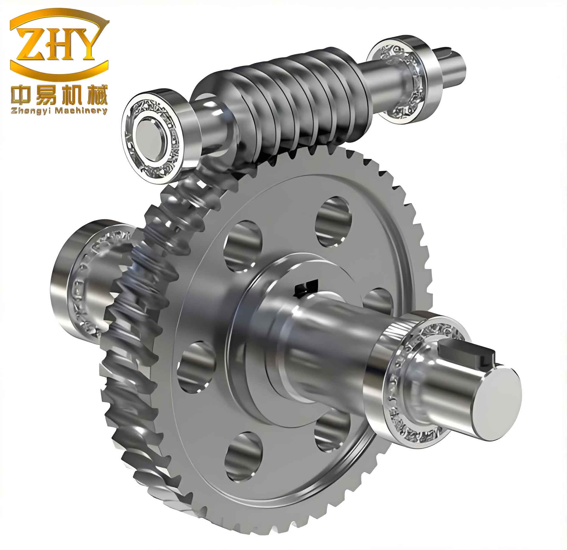
The figure shows the worm shaft, the worm wheel mounted on the vertical main shaft, and the bearing supports. The critical adjustment dimensions are:
| Parameter | Symbol | Required Tolerance | Effect if Out of Tolerance |
|---|---|---|---|
| Center distance | $a$ | ±0.05 mm | Incorrect backlash; noise; wear |
| Axial position of worm (distance from bearing to worm center) | $L$ | ±0.10 mm | Misalignment of central plane |
| Worm shaft level (inclination in Y-direction) | $\phi_y$ | ≤ 0.02 mm/m | Edge contact; rapid wheel wear |
| Verticality of main shaft | $\epsilon$ | ≤ 0.05 mm/m | Eccentric loading; vibration |
| Parallelism between worm shaft and main shaft (in X-Z plane) | $\delta$ | ≤ 0.03 mm | Non-uniform mesh |
The geometry of the meshing point can be described in a coordinate system where the worm axis is along the X-direction, the main shaft axis along the Z-direction, and Y is the radial direction. In the ideal case, the meshing point lies in the central plane (Y = 0). When the worm shaft is tilted around the X-axis by an angle $\theta$, the contact line shifts:
$$
\Delta y = L \cdot \tan\theta
$$
where $L$ is the distance from the worm support to the center of the worm wheel. Even a small tilt (e.g., $\theta = 0.1^\circ$) can cause a displacement of several millimeters, moving the contact out of the crown zone of the worm wheel.
To quantify the impact on wear, we can consider the Hertzian contact stress at the meshing point. For a misaligned contact, the stress concentration factor can be approximated by:
$$
\sigma_{\text{max}} = \sigma_0 \cdot \sqrt{\frac{r}{w}}
$$
where $\sigma_0$ is the nominal contact stress, $r$ is the radius of curvature, and $w$ is the effective width of the contact patch. When the contact is shifted to the edge of the tooth, $w$ becomes very small, and the stress increases dramatically, leading to pitting and spalling. In our factory, we observed that worm wheels that were properly installed lasted over 5 years, while those with Y-direction misalignment failed in less than 1 year.
Table 5 summarizes the most common installation errors and their consequences for worm gears.
| Error Type | Description | Effect on Worm Gears | Effect on Cement Quality |
|---|---|---|---|
| Center distance too large | $a$ exceeds tolerance | Excessive backlash; impact loading | Unsteady discharge; clinker variation |
| Center distance too small | $a$ below tolerance | Binding; overheating; seizure | Kiln stop; loss of production |
| Worm shaft not level (Y tilt) | $\phi_y > 0.02$ mm/m | Edge contact; rapid wear of worm wheel | Increased vibration; inconsistent material flow |
| Main shaft not vertical | $\epsilon > 0.05$ mm/m | Eccentric rotation; uneven loading on worm gear | Discharge fluctuation; quality non-uniformity |
| Incorrect axial position of worm | Difference from nominal $L$ | Meshing plane offset; noise | Potential damage; unpredictable maintenance |
The relationship between worm gear health and cement quality is often indirect but significant. For example, a worn worm wheel leads to uneven rotation of the discharge table, which in turn causes variations in the residence time of clinker in the kiln. This can affect the cooling rate and the final strength of the cement. Over a month, the standard deviation of the cement strength may increase by 20–30% due solely to mechanical deterioration. Therefore, maintaining precision in worm gears is not just a mechanical concern; it is a quality assurance issue.
Part III: Comprehensive Analysis Using Tables and Formulas
To provide a complete picture, I will now compare the mathematical structure of the quality indicators (CV and K) and the mechanical parameters of worm gears side by side. Although seemingly unrelated, both involve ratios and standard deviations. In quality statistics, we use $\sigma$ to represent dispersion; in worm gear theory, we use center distance tolerance $\delta a$ to represent manufacturing accuracy. The following table draws an analogy.
| Quality Indicator | Formula | Worm Gear Parameter | Formula |
|---|---|---|---|
| Coefficient of variation (CV) | $\sigma / \mu$ | Relative center distance variation | $\delta a / a$ |
| Guarantee coefficient (K) | $(\mu – X_{\min}) / \sigma$ | Safety margin against tooth interference | $(a – a_{\min}) / \delta a$ |
| Standard deviation $\sigma$ | Measure of spread | Manufacturing tolerance $\delta a$ | Measure of deviation |
| Target mean $\mu$ | Design strength | Nominal center distance $a$ | Design geometry |
| Minimum specification $X_{\min}$ | Lower limit | Minimum allowable center distance $a_{\min}$ | Lower limit for safe operation |
This analogy shows that the same kind of thinking – balancing mean, variability, and a lower bound – applies to both fields. In cement quality, we want $\mu$ high and $\sigma$ low; in worm gear installation, we want $a$ exactly at nominal and $\delta a$ small.
For a deeper mathematical treatment, consider the probability that the compressive strength of a cement batch falls below the minimum. Assuming a normal distribution, the probability is:
$$
P_{\text{fail}} = \Phi\left( -\frac{\mu – X_{\min}}{\sigma} \right) = \Phi(-K)
$$
where $\Phi$ is the standard normal CDF. Thus, K directly determines the failure probability. Similarly, for worm gears, the probability of interference (tooth contact outside the allowed zone) can be related to a tolerance index:
$$
P_{\text{interference}} = \Phi\left( -\frac{a – a_{\min}}{\sigma_a} \right)
$$
where $\sigma_a$ is the standard deviation of the center distance due to manufacturing and installation errors. Again, a larger “gear guarantee coefficient” $K_G = (a – a_{\min}) / \sigma_a$ reduces the risk of interference.
Table 7 provides a comparison of typical values observed in our factory for cement quality and worm gear installation.
| Parameter | Cement Quality (Monthly) | Worm Gear Installation |
|---|---|---|
| Target value | $\mu = 48$ MPa (for 42.5 grade) | $a = 200$ mm (nominal) |
| Standard deviation / tolerance | $\sigma = 2.0$ MPa | $\delta a = 0.05$ mm (installation tolerance) |
| Lower limit | $X_{\min} = 42.5$ MPa | $a_{\min} = 199.8$ mm (from design) |
| Guarantee coefficient | $K = (48-42.5)/2 = 2.75$ | $K_G = (200-199.8)/0.05 = 4.0$ |
| Failure/interference probability | $\Phi(-2.75) \approx 0.003$ | $\Phi(-4.0) \approx 0.00003$ |
From this, we see that a well-maintained worm gear installation can achieve a failure probability three orders of magnitude lower than typical cement quality risk. However, if the worm gear installation is neglected, the effective tolerance $\delta a$ can increase (e.g., due to wear or misalignment), lowering $K_G$ and increasing the risk of mechanical failure. This mechanical failure then cascades into causing larger $\sigma$ in cement strength, because the kiln operation becomes unstable.
Part IV: Detailed Installation Procedures for Worm Gears
Based on my experience, I recommend the following step-by-step installation procedure for worm gears in vertical shaft kilns, with emphasis on the Y-direction leveling:
- Foundation preparation: Ensure the base plate is flat within 0.02 mm/m. Use shims to adjust.
- Mount the worm wheel assembly: Install the worm wheel on the main shaft. Check the verticality of the main shaft using a dial indicator at four points around the circumference. The maximum deviation should be ≤ 0.05 mm/m.
- Position the worm housing: Place the worm housing on the base. Using a precision level, adjust the worm shaft to be horizontal in both the X and Y directions. The Y-direction level is often the most neglected: use a frame level on the ground surfaces of the housing to achieve ≤ 0.02 mm/m.
- Check the center distance: Measure $a$ with a micrometer inside gauge. Adjust the position of the worm housing until $a$ is within ±0.05 mm of the nominal value.
- Axial alignment: Ensure the axial center of the worm coincides with the center of the worm wheel width. Use a feeler gauge or a depth micrometer to measure the gap between the worm face and the wheel side. The difference should be ≤ 0.10 mm.
- Backlash check: Rotate the worm wheel by hand; measure the backlash at several points around the circumference. For globoid worm gears, the recommended backlash is 0.1–0.3 mm, depending on the module.
- Paint contact test: Apply a thin coat of Prussian blue to the worm threads. Rotate the worm under light load. Examine the contact pattern on the worm wheel teeth. The pattern should be centrally located, covering at least 60% of the tooth width. If the pattern is at the edge, recheck the Y-direction level and axial position.
- Final tightening: Tighten all bolts to the specified torque using a torque wrench. Re-measure all critical dimensions after tightening, because even slight shifts can occur.
Table 8 summarizes the tools and tolerances for each step.
| Installation Step | Tool | Target Tolerance |
|---|---|---|
| Base flatness | Precision straightedge + feeler gauge | ≤ 0.02 mm/m |
| Main shaft verticality | Dial indicator (magnetic base) | ≤ 0.05 mm/m |
| Worm shaft Y-level | Frame level (0.02 mm/m accuracy) | ≤ 0.02 mm/m |
| Center distance | Inside micrometer (range 0–300 mm) | ±0.05 mm |
| Axial position | Depth micrometer | ±0.10 mm |
| Backlash | Dial indicator on worm wheel tooth | 0.1–0.3 mm |
| Contact pattern | Prussian blue | Central, >60% width |
After installation, regular maintenance of worm gears is essential. Every three months, inspect the contact pattern again, measure the backlash, and check for any signs of pitting or abrasion on the worm wheel teeth. The wear rate can be monitored by measuring the thickness of the tooth at the pitch line. The allowable wear limit is typically 10% of the original tooth thickness. Beyond that, the worm wheel should be replaced.
Part V: Extended Discussion on Worm Gear Materials and Lubrication
The material selection for worm gears is another critical factor. In our factory, the worm is made of 40Cr forged steel, hardened and tempered to HRC 45–50, while the worm wheel is made of ductile iron (QT500-7). This combination provides a good balance between strength and wear resistance, but it is sensitive to misalignment. If the Y-direction level is off, the harder worm will quickly cut into the softer wheel.
Lubrication also plays a vital role. For globoid worm gears, we recommend a synthetic gear oil with EP (extreme pressure) additives, with a viscosity grade of ISO VG 460. The oil should be filtered to prevent particles from accelerating wear. The oil sump temperature should be monitored; if it exceeds 80°C, the oil degrades faster and the risk of scuffing increases. The heat generation in worm gears can be estimated by:
$$
Q = P \cdot (1 – \eta)
$$
where $P$ is the input power and $\eta$ is the efficiency. For a globoid worm gear, $\eta$ typically ranges from 0.75 to 0.90. The efficiency itself is a function of the lead angle $\gamma$ and the coefficient of friction $\mu_f$:
$$
\eta = \frac{\tan\gamma}{\tan(\gamma + \arctan\mu_f)}
$$
Thus, a small lead angle (high reduction ratio) yields lower efficiency and more heat. Proper installation ensures that $\mu_f$ remains low (good lubricant film) and that the contact stresses are minimized.
To further illustrate the relationship between worm gear parameters and performance, I have compiled Table 9 showing typical globoid worm gear data for our VSK.
| Parameter | Symbol | Value |
|---|---|---|
| Center distance | $a$ | 200 mm |
| Worm pitch diameter | $d_1$ | 80 mm |
| Worm wheel pitch diameter | $d_2$ | 320 mm |
| Number of worm threads | $z_1$ | 2 |
| Number of worm wheel teeth | $z_2$ | 40 |
| Reduction ratio | $i = z_2 / z_1$ | 20 |
| Axial module | $m$ | 8 mm |
| Lead angle | $\gamma$ | 11.3° |
| Pressure angle | $\alpha$ | 20° |
| Input power | $P$ | 15 kW |
| Input speed | $n_1$ | 1450 rpm |
| Output torque | $T_2$ | ≈ 4000 Nm |
The reduction ratio formula:
$$
i = \frac{n_1}{n_2} = \frac{z_2}{z_1}
$$
For this gear set, the worm wheel rotates at $n_2 = 72.5$ rpm. The slow rotation, combined with the self-locking feature (lead angle < friction angle), ensures that the discharge table does not freewheel if power is lost.
Part VI: Conclusion and Recommendations
After years of working with cement quality and mechanical equipment, I have come to the following conclusions:
- The coefficient of variation (CV) and the guarantee coefficient (K) are mathematically equivalent in the sense that both are functions of $\mu$ and $\sigma$. However, they provide complementary information: CV shows relative dispersion, while K shows the safety margin relative to the minimum specification. Neither is inherently “more scientific” than the other; they should be used together.
- In practice, K can indirectly indicate potential quality risks when the mean is close to the lower limit, even if CV is small. Conversely, a large K with a high CV may still hide excessive variability. Thus, a balanced evaluation requires both indicators.
- The installation of worm gears in vertical shaft kilns is a critical factor that directly affects the mechanical reliability and, consequently, the consistency of cement quality. The often-neglected Y-direction leveling of the worm shaft must be given the same attention as the verticality of the main shaft and center distance.
- Using the analogies between quality statistics and gear geometry, I have shown that a “gear guarantee coefficient” can be defined and that proper installation reduces the risk of mechanical failure to extremely low levels, which in turn helps keep the cement strength variability low.
- Regular maintenance and monitoring of worm gears, including contact pattern checks and backlash measurements, are essential to sustain high cement quality. The cost of replacing a worm wheel due to misalignment is much higher than the cost of precise installation.
I encourage all quality engineers to not only analyze statistical indicators but also to physically inspect the condition of their worm gears and other critical drives. In my experience, the correlation between mechanical health and final product quality is undeniable. By combining robust statistical process control with meticulous mechanical maintenance, we can achieve cement that is not only statistically capable but also consistently reliable.
To summarize, I have provided a comprehensive discussion with 9 tables and numerous formulas covering both cement quality indicators and worm gear installation. The key message is that both domains benefit from an understanding of variability, tolerance, and safety margins. Whether we are evaluating the coefficient of variation or setting the Y-direction level of a worm gear, the underlying principles of measurement and control remain the same.