
The pursuit of intelligent manufacturing and the advancement of industrial robotics have placed critical demands on the reliability and health management of core components. Among these, the RV reducer stands as a pivotal precision transmission unit within robotic joints, known for its high reduction ratio, compact structure, and significant load-bearing capacity. The operational integrity of the RV reducer is paramount to the performance and longevity of the entire robotic system. However, the complex internal structure involving components like the cycloid gear, planet gears, and needle pins makes the RV reducer susceptible to various failure modes such as pitting and wear. The vibration signals generated by these faults are often non-stationary and non-linear, making their diagnosis a challenging task. Traditional fault diagnosis methods frequently rely on extensive feature engineering and shallow machine learning models, which may not fully capture the intricate patterns within the signal data. This work explores the application of a deep learning architecture, specifically the Residual Network (ResNet), to directly and effectively classify fault conditions of the RV reducer using raw vibration signals.
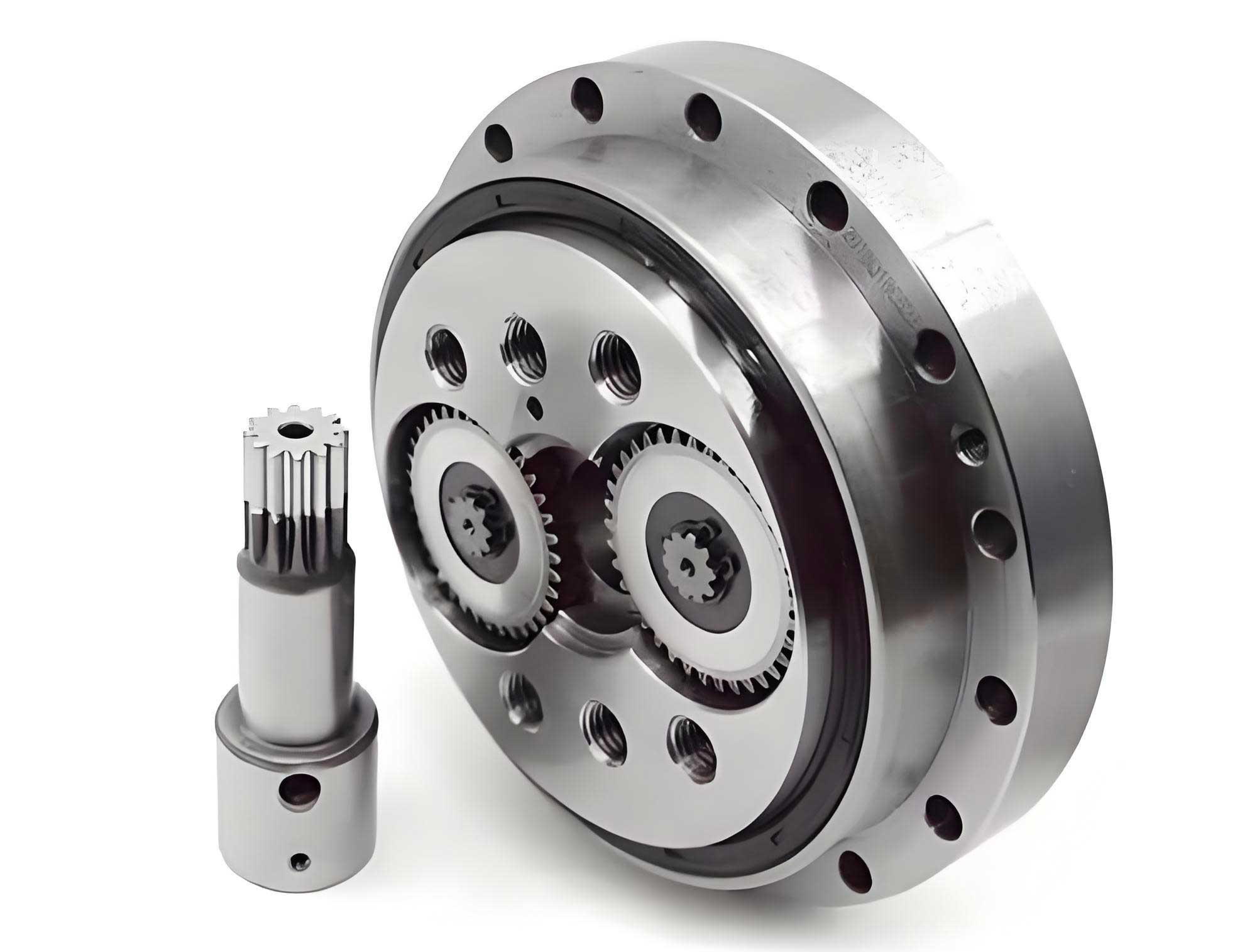
The core contribution of this approach lies in leveraging the powerful feature extraction and hierarchical learning capabilities of deep residual networks. The model is designed to accept preprocessed two-dimensional signal maps as input, automatically learn discriminative features through multiple convolutional layers and residual blocks, and perform accurate multi-class classification. This method significantly reduces the reliance on manual feature design. The performance of the proposed model is rigorously validated using vibration data collected from a dedicated RV reducer test rig under multiple operating conditions and fault types. Comparisons with other neural network architectures demonstrate the superiority of the ResNet model in diagnosing faults in the complex RV reducer system.
Residual Network Architecture for Signal Classification
The selected model is a deep convolutional neural network built upon the residual learning framework. This architecture is chosen to mitigate the vanishing gradient problem commonly encountered when training very deep networks, thereby enabling effective training and superior performance. The network consists of an initial convolutional layer, followed by a series of four residual blocks, and concludes with global average pooling and a fully connected classification layer. The overall architecture facilitates the automatic learning of spatial hierarchies of features from the input signal maps.
The fundamental building block of this network is the residual unit. For a given input $\mathbf{x}$ to a residual block, the block learns a residual mapping $\mathcal{F}(\mathbf{x})$ rather than the desired underlying mapping $\mathcal{H}(\mathbf{x})$. The original mapping is recast as $\mathcal{H}(\mathbf{x}) = \mathcal{F}(\mathbf{x}) + \mathbf{x}$. This is realized via a shortcut connection that performs identity mapping and adds its output to the output of the stacked convolutional layers. This simple addition operation allows gradients to flow directly through the shortcut connections during backpropagation, alleviating degradation issues. The operations within a standard residual block can be summarized as:
$$\mathbf{y} = \sigma(\mathcal{F}(\mathbf{x}, \{W_i\}) + \mathbf{x})$$
where $\mathbf{x}$ and $\mathbf{y}$ are the input and output vectors of the block, $\mathcal{F}(\mathbf{x}, \{W_i\})$ represents the residual mapping to be learned (e.g., two convolutional layers), and $\sigma$ denotes the ReLU activation function. For blocks where the input and output dimensions differ, a linear projection $W_s$ is performed on the shortcut connection to match dimensions: $\mathbf{y} = \sigma(\mathcal{F}(\mathbf{x}, \{W_i\}) + W_s \mathbf{x})$.
The specific parameters for the convolutional layers within the residual blocks are detailed in Table 1. The use of stride 2 in the second convolutional layer of Block2 performs down-sampling, reducing the spatial dimensions of the feature maps and the computational load for subsequent layers.
| Residual Block | Parameters for Conv1 | Parameters for Conv2 |
|---|---|---|
| Block1 | Conv(3,3,1,64) | Conv(3,3,1,64) |
| Block2 | Conv(3,3,1,64) | Conv(3,3,2,64) |
| Block3 | Conv(3,3,1,128) | Conv(3,3,1,128) |
| Block4 | Conv(3,3,1,256) | Conv(3,3,1,256) |
Non-linearity is introduced via the Rectified Linear Unit (ReLU) activation function, defined as:
$$ \text{ReLU}(x) = \max(0, x) $$
This function is applied after each convolutional layer. The final layer utilizes the Softmax function to output a probability distribution over the fault classes. For an input vector $\mathbf{z}$ of length $n$, the probability for class $i$ is:
$$ S_i = \frac{e^{z_i}}{\sum_{j=1}^{n} e^{z_j}} $$
The class with the highest probability is selected as the diagnostic prediction.
Vibration Signal Acquisition and Preprocessing
Data acquisition is fundamental for developing a data-driven diagnostic model. Vibration signals were collected from an RV reducer operating under controlled conditions on a dedicated test bench. The system consisted of a servo motor driving the RV reducer, with a magnetic powder brake applying variable load torque. An accelerometer was mounted on the housing of the RV reducer to capture axial vibration signals. Experiments were conducted under a constant input speed and multiple load levels, as outlined in Table 2. The objective was to capture a representative dataset encompassing various operational states.
| Parameter | Value |
|---|---|
| Motor Speed (r/min) | 400 |
| Reducer Load (N·m) | 0, 20, 40, 60, 80, 100, 120 |
| Sampling Frequency (Hz) | 2000 |
To evaluate the diagnostic capability, five distinct health states of the RV reducer were considered, including one normal state and four fault states. The fault states comprised single-component pitting and compound faults involving multiple components, as defined in Table 3. Compound faults present a greater diagnostic challenge, providing a rigorous test for the model.
| Label | RV Reducer Condition |
|---|---|
| 0 | Normal (No Fault) |
| 1 | Planet Gear Pitting |
| 2 | Cycloid Gear Pitting |
| 3 | Planet Gear Pitting + Pin Pitting |
| 4 | Cycloid Gear Pitting + Pin Pitting |
Raw vibration signals required significant preprocessing before being fed into the residual network. The key steps were:
1. Normalization: Each individual signal sample was normalized to a [0, 1] range to ensure stable and efficient network training. For a signal sample $x$,
$$ y = \frac{x – \min(x)}{\max(x) – \min(x)} $$
2. Dataset Construction & Augmentation: The continuous vibration signal for each condition was segmented into overlapping samples of fixed length (1024 data points). Using a step size smaller than the sample length (e.g., 170) created an augmented training set, increasing the number of training instances and improving model robustness.
3. Dimensionality Transformation: Convolutional neural networks are inherently designed for two-dimensional input (like images). Therefore, each 1D signal vector of length $L=1024$ was reshaped into a 2D matrix. A simple and effective row-wise stacking method was employed. For example, to create a 32×32 matrix, the first 32 points form the first row, the next 32 points the second row, and so on. The impact of different reshaping dimensions (e.g., 32×32, 64×16, 128×8) on diagnostic accuracy was investigated.
Experimental Results and Model Performance
The prepared dataset was split into training and testing sets. The model was trained using the Adam optimizer, with a carefully scheduled learning rate starting at 0.0001 for pre-training and adjusting during training for optimal convergence. The loss function was categorical cross-entropy, and training was performed for a sufficient number of epochs until both training and validation metrics stabilized.
The primary performance metric is classification accuracy. The residual network model achieved a high level of performance on the RV reducer fault diagnosis task. To ensure a robust evaluation and prevent overfitting, a 5-fold cross-validation procedure was repeated three times. The results, presented in Table 4, show a consistent average testing accuracy of approximately 98.11%, while training accuracy reached near 100%. This small gap indicates the model generalizes well to unseen data from the RV reducer.
| Trial | Fold Number | Avg. Test Acc. | ||||
|---|---|---|---|---|---|---|
| 1 | 2 | 3 | 4 | 5 | ||
| 1 (Train) | 100 | 100 | 100 | 100 | 100 | 98.11 |
| 1 (Test) | 98.59 | 97.85 | 98.06 | 97.85 | 98.26 | |
| 2 (Train) | 100 | 99.61 | 100 | 100 | 100 | |
| 2 (Test) | 98.43 | 97.83 | 98.06 | 97.93 | 98.36 | 98.12 |
| 3 (Train) | 100 | 100 | 100 | 100 | 100 | 98.09 |
| 3 (Test) | 98.47 | 97.76 | 98.13 | 97.90 | 98.17 | |
An interesting finding was the influence of the 1D-to-2D signal reshaping strategy. As shown in Table 5, the configuration of the 2D matrix (rows x columns) significantly impacted the final accuracy. Reshaping the 1024-point signal into a 128×8 matrix (more rows than columns) yielded the best performance, with an average accuracy exceeding 99.1%. This suggests that the spatial correlations learned by the convolutional kernels are sensitive to the structural arrangement of the temporal signal data.
| Rows | Columns | Trial 1 Acc. | Trial 2 Acc. | Trial 3 Acc. | Average Acc. |
|---|---|---|---|---|---|
| 8 | 128 | 91.77 | 92.11 | 91.67 | 91.85 |
| 16 | 64 | 94.19 | 94.46 | 94.27 | 94.31 |
| 32 | 32 | 98.12 | 98.12 | 98.09 | 98.11 |
| 64 | 16 | 99.27 | 99.19 | 98.89 | 99.12 |
| 128 | 8 | 99.29 | 99.19 | 99.10 | 99.19 |
To demonstrate the generalizability of the proposed residual network architecture beyond the specific RV reducer dataset, it was applied to a publicly available bearing fault dataset (Case Western Reserve University Bearing Data Center). The model, with the same architecture but trained on bearing vibration signals processed identically, achieved an average accuracy of 99.49% in classifying bearing health states. This confirms that the residual network is a versatile and powerful tool for mechanical fault diagnosis from vibration signals.
Comparative Analysis and Feature Visualization
The performance of the proposed ResNet model was compared against other neural network models to highlight its advantages for RV reducer fault diagnosis. The compared models included a standard Deep Neural Network (DNN) with fully connected layers, the classic LeNet-5 convolutional network, and a 10-layer plain Convolutional Neural Network (CNN) without residual connections. The results of 5-fold cross-validation for these models are summarized in Table 6. The DNN performed poorly, struggling to learn from the raw signal data without convolutional feature extraction. LeNet showed improved performance but was limited by its shallow depth. The 10-layer CNN performed better but was still surpassed by the ResNet model. The ResNet’s superior accuracy, particularly over the plain 10-layer CNN, underscores the effectiveness of the residual shortcut connections in enabling the training of a deeper, more capable network for this complex diagnostic task involving the RV reducer.
| Model | Trial 1 Avg. | Trial 2 Avg. | Trial 3 Avg. | Overall Average |
|---|---|---|---|---|
| Deep Neural Network (DNN) | 62.69 | 63.07 | 62.42 | 62.73 |
| LeNet-5 | 86.42 | 86.38 | 86.71 | 86.50 |
| 10-Layer CNN (Plain) | 95.86 | 95.57 | 95.47 | 95.63 |
| Proposed ResNet (32×32) | 98.12 | 98.12 | 98.09 | 98.11 |
To gain insight into the internal feature learning process of the residual network, a dimensionality reduction technique was applied to the high-dimensional feature vectors extracted from the global average pooling layer. Linear Discriminant Analysis (LDA) was used to project these 256-dimensional features onto a 3D space for visualization. The evolution of these feature clusters at different training stages is instructive. At initialization (iteration 0), features from all RV reducer health states are randomly intermixed. After partial training (e.g., 4500 iterations), clusters begin to form, but significant overlap remains, especially among the more challenging compound fault classes (Label 3 and 4). Upon full convergence (8000 iterations), the features form well-separated, compact clusters corresponding to each fault type. This visual progression confirms that the residual network successfully learns highly discriminative representations that linearly separate the different conditions of the RV reducer. The visualization also aligns with the quantitative results, showing that compound faults are indeed more challenging to separate than single faults.
Conclusion
This work presents a robust and effective deep-learning-based framework for the fault diagnosis of the RV reducer. The application of a Residual Network model directly to preprocessed two-dimensional vibration signal maps eliminates the need for manual feature extraction, streamlining the diagnostic pipeline. The model demonstrated exceptional performance, achieving an average classification accuracy of 98.11% for five health states of the RV reducer, including challenging compound faults. The superiority of the ResNet architecture was validated through comparisons with DNN, LeNet, and a plain deep CNN, with the residual connections proving crucial for achieving high accuracy. Furthermore, the model showed strong generalizability when tested on a standard bearing fault dataset. The study also revealed that the method used to reshape the 1D time-series signal into a 2D matrix is a significant hyperparameter, with certain configurations (e.g., 128×8) further boosting performance. Visualization of the learned features via LDA provided intuitive confirmation of the model’s discriminative capability. In summary, the proposed residual network offers a powerful, accurate, and generalizable solution for the intelligent fault diagnosis of complex mechanical systems like the RV reducer, contributing to the advancement of predictive maintenance for robotic and precision industrial applications.