
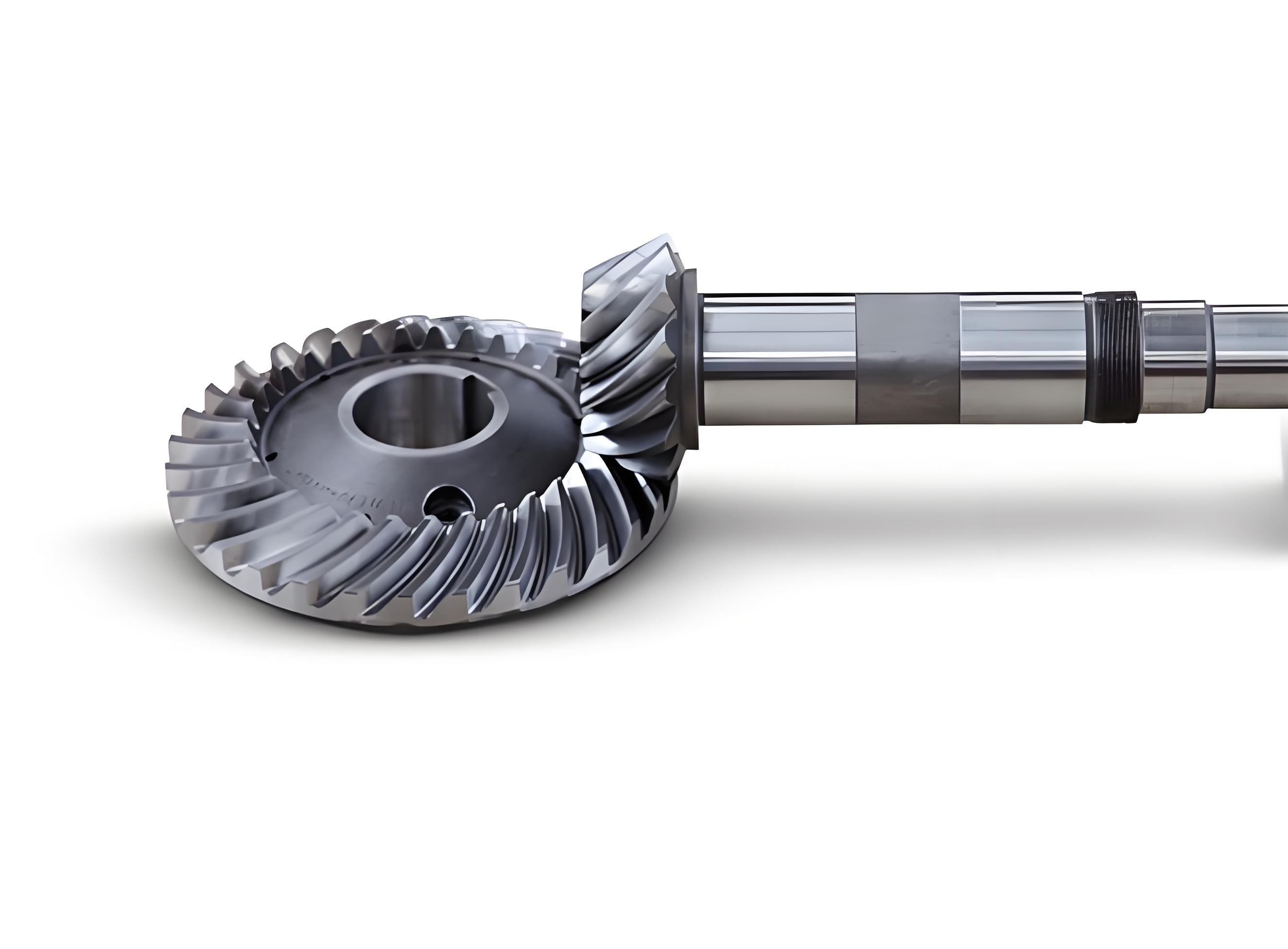
Ensuring the reliable operation of mechanical transmission systems is paramount in industries such as aviation, automotive, and maritime. Among critical components, spiral bevel gears are favored for their high load-bearing capacity, efficiency, and stable transmission ratios. However, their operation in harsh conditions like heavy loads and enclosed spaces makes them susceptible to failures. A fault in a spiral bevel gear can cascade through the entire drive chain, leading to significant economic losses and safety hazards. Therefore, developing effective fault diagnosis methods for spiral bevel gears is crucial for predictive maintenance and operational safety.
The vibration signals generated by faulty spiral bevel gears are inherently complex. Compared to spur gears, their wider contact surfaces and continuous tooth engagement during meshing produce signals characterized by strong background noise, pronounced nonlinearity, and non-stationary behavior. Traditional time-domain or frequency-domain analysis techniques often struggle to extract meaningful fault features from such noisy, complex signals. This necessitates the use of more advanced signal processing tools capable of preserving phase information and suppressing noise.
Higher-order spectral analysis, specifically bispectral analysis, offers a powerful solution. The bispectrum, being a third-order statistic, retains full information about the signal’s amplitude, frequency, and phase. It possesses properties like time-shift invariance and phase preservation, and most importantly, it can suppress Gaussian colored noise. This makes it exceptionally suitable for analyzing the challenging vibration signals from spiral bevel gears. However, the conventional bispectrum is a two-dimensional symmetric plot, leading to significant data redundancy. Feeding the full bispectrum into a diagnostic model increases computational load without adding unique information. This work proposes the use of a local bispectrum—a specific, non-redundant portion of the full bispectrum—as an optimal input feature.
For the classification stage, shallow machine learning models like Support Vector Machines (SVM) or Backpropagation (BP) Neural Networks have been widely used. These models, however, are often limited in their ability to automatically learn complex, hierarchical features from raw data, requiring extensive manual feature engineering. Convolutional Neural Networks (CNNs), a class of deep learning models, excel at automatic feature extraction from structured data like images. Their hierarchical structure allows them to learn low-level features (e.g., edges, textures) and combine them into high-level, discriminative patterns directly from the input. This study integrates the feature representation power of the local bispectrum with the pattern recognition capability of a CNN to create a robust, efficient, and accurate fault diagnosis framework for spiral bevel gears.
Theoretical Foundations
1. Bispectral Analysis
Given a zero-mean, real-valued stationary random signal sequence ${x(n)}$, its third-order cumulant (or moment) is defined as:
$$R(\tau_1, \tau_2) = E\{x(n)x(n+\tau_1)x(n+\tau_2)\}$$
where $E\{\cdot\}$ denotes the mathematical expectation, and $\tau_1$, $\tau_2$ are time lags. The bispectrum, $B(\omega_1, \omega_2)$, is defined as the two-dimensional Fourier transform of this third-order cumulant:
$$B(\omega_1, \omega_2) = \sum_{\tau_1=-\infty}^{\infty} \sum_{\tau_2=-\infty}^{\infty} R(\tau_1, \tau_2) e^{-j(\omega_1\tau_1 + \omega_2\tau_2)}$$
where $\omega_1$ and $\omega_2$ are angular frequencies. A practical estimator for the bispectrum, based on the Fourier transforms of signal segments, is given by:
$$B(\omega_1, \omega_2) = X(\omega_1) X(\omega_2) X^*(\omega_1 + \omega_2)$$
Here, $X(\omega)$ is the Discrete-Time Fourier Transform (DTFT) of $x(n)$, and $*$ denotes the complex conjugate. The bispectrum is complex-valued and exhibits several symmetries. For real signals, it is fully defined within a triangular region in the frequency plane $(\omega_1, \omega_2)$ satisfying $0 \le \omega_2 \le \omega_1$, $\omega_1 + \omega_2 \le \pi$. The magnitude of the bispectrum, $|B(\omega_1, \omega_2)|$, reveals quadratic phase couplings between frequency components, which are often indicative of nonlinear interactions caused by faults in mechanical systems like spiral bevel gears.
2. From Full to Local Bispectrum
The symmetry of the bispectrum implies that the information contained in the full $N \times N$ bispectral matrix is highly redundant. Using the entire matrix as an input to a classifier, such as a CNN, is computationally inefficient. It forces the network to learn the same patterns multiple times across symmetric regions, wasting model capacity and training time. The concept of the local bispectrum addresses this. By extracting only the non-redundant principal region—typically the triangular or wedge-shaped region defined by $\omega_2 \le \omega_1$ and $\omega_1 + \omega_2 \le f_s/2$ (where $f_s$ is the sampling frequency)—we obtain a compact representation. In practice, this is often implemented by taking the top-left quadrant of the magnitude bispectrum plot. This local bispectrum retains all the unique phase coupling information of the original signal while reducing the input dimensionality significantly. For a spiral bevel gear vibration signal, this translates to a concise yet information-rich 2D image that encapsulates the fault-induced nonlinear characteristics.
3. Convolutional Neural Networks (CNN)
A typical CNN architecture is composed of an input layer, multiple convolutional and pooling layers, followed by one or more fully connected layers and an output layer. The core operations are as follows:
Convolutional Layers: These layers apply a set of learnable filters (kernels) to the input. Each filter slides across the input (e.g., the local bispectrum image) performing element-wise multiplication and summation, producing a feature map. This operation allows the network to detect local patterns like edges, corners, and textures. The output of the $l$-th convolutional layer for the $j$-th feature map is computed as:
$$a^l_j = \sigma \left( \sum_{i \in M_j} a^{l-1}_i * \omega^l_{ij} + b^l_j \right)$$
where $a^{l-1}_i$ is the input from the $i$-th feature map in the previous layer, $M_j$ is the set of input maps, $*$ denotes the convolution operation, $\omega^l_{ij}$ is the kernel weight matrix, $b^l_j$ is the bias, and $\sigma(\cdot)$ is a non-linear activation function like the Rectified Linear Unit (ReLU).
Pooling Layers: Pooling (or subsampling) layers follow convolutional layers to reduce the spatial dimensions of the feature maps, providing translation invariance and decreasing computational complexity. Max pooling, which outputs the maximum value in a local region (e.g., a 2×2 window), is commonly used.
Fully Connected Layers: After several cycles of convolution and pooling, the high-level feature maps are flattened into a one-dimensional vector and fed into fully connected layers. These layers perform high-level reasoning and combine the learned features for the final classification task.
Output Layer: The final layer typically uses a softmax activation function for multi-class classification, outputting a probability distribution over the possible fault states of the spiral bevel gear (e.g., healthy, cracked, broken tooth).
The training process involves forward propagation of an input (like a local bispectrum), calculation of a loss function (e.g., cross-entropy), and backward propagation of errors to update the weights ($\omega$) and biases ($b$) via gradient descent optimization algorithms like Adam.
The Proposed Diagnostic Methodology
The proposed framework for spiral bevel gear fault diagnosis synergistically combines local bispectral analysis and CNN-based pattern recognition. The complete workflow is systematically presented below and can be summarized in the following major steps:
| Step | Description | Key Action |
|---|---|---|
| 1 | Data Acquisition & Segmentation | Collect vibration signals from the spiral bevel gearbox under various health states. Segment the long-time signal into multiple non-overlapping samples of fixed length $L$. |
| 2 | Local Bispectrum Generation | For each data segment $x_i(n)$ of length $L$, compute its bispectrum $B_i(\omega_1, \omega_2)$. Extract the non-redundant region to form the local bispectrum image $LB_i$. |
| 3 | Dataset Construction | Assign a class label (fault type) to each $LB_i$. Split the collection of all labeled $LB_i$ into training and testing sets. |
| 4 | CNN Model Configuration | Design the CNN architecture (number of layers, filter sizes, etc.). Initialize hyperparameters (learning rate, batch size, number of epochs). |
| 5 | Model Training | Feed the training set local bispectrum images into the CNN. Iteratively adjust network parameters via backpropagation to minimize classification error. |
| 6 | Model Evaluation & Diagnosis | Input the unseen test set local bispectrum images into the trained CNN model. The model outputs a predicted fault class for each test sample, enabling automatic diagnosis. |
The strength of this methodology lies in the complementary roles of its two core components. The local bispectrum acts as a powerful pre-processor that transforms the complex, noisy 1D vibration signal from the spiral bevel gear into a cleaner, more informative 2D image representation. It inherently suppresses noise and highlights the nonlinear phase-coupled components associated with faults. Subsequently, the CNN serves as an intelligent classifier that automatically learns the distinct visual patterns within these local bispectrum images corresponding to different fault conditions of the spiral bevel gear, without requiring manual feature design.
Experimental Validation and Analysis
1. Spiral Bevel Gear Test Rig and Data Description
To validate the proposed method, a spiral bevel gear fault simulation experiment was conducted. Vibration data was acquired from a spiral bevel gear reduction box test rig using an accelerometer mounted on the input shaft. Data was collected at a sampling frequency of 8192 Hz with an input shaft speed of 1200 rpm. Four distinct health states of the driving spiral bevel gear were considered:
- State 1 (Healthy): Gear with no defects.
- State 2 (Root Crack): Gear with a fatigue crack at the tooth root.
- State 3 (1/3 Broken Tooth): Gear with approximately one-third of a tooth missing.
- State 4 (2/3 Broken Tooth): Gear with approximately two-thirds of a tooth missing.
For each state, the raw vibration signal was partitioned into 500 non-overlapping segments, each containing 1024 data points. This resulted in a total of 2000 data samples (500 samples × 4 states).
2. Generation of Local Bispectrum CNN Inputs
Each 1024-point vibration segment was processed to generate its bispectrum. The magnitude of the bispectrum was computed and plotted as a 2D image. Subsequently, the top-left quadrant (128×128 pixels) of this image was cropped to form the local bispectrum sample. This process converted each 1D time-series sample into a 2D grayscale image perfectly suited for CNN processing. From the total 2000 samples, 600 samples (150 per state) were randomly selected to form the training set, and the remaining 1400 samples (350 per state) constituted the independent test set.
3. CNN Architecture and Training Parameters
A custom CNN model was constructed for this diagnosis task. The detailed architecture is specified in the table below.
| Layer Type | Output Shape / #Maps | Kernel/Pool Size | Stride | Activation / Notes |
|---|---|---|---|---|
| Input Layer | 128 × 128 × 1 | – | – | Local Bispectrum Image |
| Conv2D (C1) | 128 × 128 × 8 | 3 × 3 | 1 × 1 | ReLU |
| MaxPooling2D (P1) | 64 × 64 × 8 | 2 × 2 | 2 × 2 | – |
| Conv2D (C2) | 64 × 64 × 16 | 3 × 3 | 1 × 1 | ReLU |
| MaxPooling2D (P2) | 32 × 32 × 16 | 2 × 2 | 2 × 2 | – |
| Conv2D (C3) | 32 × 32 × 32 | 3 × 3 | 1 × 1 | ReLU |
| Flatten Layer | 32768 | – | – | – |
| Fully Connected (F) | 4 | – | – | Softmax (Output) |
The model was trained using the Adam optimizer with a learning rate of 0.0001, a batch size of 50, and for 60 epochs. The training process showed rapid convergence, with the accuracy on the training set reaching approximately 99.5% and the loss approaching zero by the final epoch.
4. Diagnostic Results and Comparative Study
The performance of the proposed Local Bispectrum + CNN method was rigorously evaluated and compared against four other diagnostic approaches to demonstrate its superiority for spiral bevel gear fault diagnosis:
- Full Bispectrum + CNN: Using the complete symmetric bispectrum image as CNN input.
- Raw Vibration Signal + CNN: Using the 1D raw vibration signal segment as input to a 1D-CNN.
- Local Bispectrum + SVM: Using the flattened local bispectrum vector as features for a Support Vector Machine classifier with RBF kernel.
- Local Bispectrum + BP Network: Using the flattened local bispectrum vector as input to a traditional Backpropagation Neural Network.
To ensure statistical reliability, each comparative experiment was repeated 100 times, and the average performance metrics were recorded. The key results are consolidated in the table below.
| Diagnosis Method | Average Diagnosis Accuracy (%) | Average Model Training Time (seconds) | Key Observations |
|---|---|---|---|
| Local Bispectrum + CNN (Proposed) | 99.56 | 15 | Highest accuracy with fastest training time among deep learning methods. Optimal balance. |
| Full Bispectrum + CNN | 99.53 | 78 | Similar high accuracy, but training time ~5x longer due to redundant input data. |
| Raw Vibration Signal + CNN | 92.65 | 18 | Fast training but significantly lower accuracy. 1D signal contains too much noise for CNN to learn robust features directly. |
| Local Bispectrum + SVM | 98.03 | 2763 | Accuracy close to proposed method, but training time is prohibitively long (~184x slower). SVM training complexity scales poorly. |
| Local Bispectrum + BP Network | 88.91 | 631 | Lowest accuracy and slow training. Shallow BP network cannot effectively learn complex patterns from the bispectral images. |
Analysis of Results:
- Efficacy of Local Bispectrum: Comparing the first two methods clearly shows the advantage of the local bispectrum. It achieves virtually identical diagnostic accuracy as the full bispectrum while reducing the CNN training time by approximately 80%. This confirms that the local bispectrum successfully eliminates redundancy without losing discriminative fault information related to the spiral bevel gear’s condition.
- Superiority of the CNN Classifier: The comparison between Local Bispectrum + CNN and Local Bispectrum + SVM/BP highlights the strength of the deep learning approach. While SVM achieved good accuracy, its training time was orders of magnitude higher, making it impractical for real-world applications or model re-tuning. The CNN, with its parameter-sharing convolutional structure and efficient gradient-based training, learns a powerful classifier much faster. The poor performance of the BP network underscores the limitation of shallow architectures in handling complex image-like inputs for spiral bevel gear fault diagnosis.
- Importance of Feature Extraction: The poor performance of Raw Vibration Signal + CNN (92.65% accuracy) versus the proposed method (99.56%) is striking. It demonstrates that feeding raw, noisy signals directly into a CNN is suboptimal. The local bispectrum serves as a crucial preprocessing step that transforms the data into a format where fault-related features are enhanced and noise is suppressed, enabling the CNN to learn more effectively and generalize better. This transformation is particularly vital for the non-stationary, nonlinear signals from spiral bevel gears.
The confusion matrix for a single run of the proposed method on the test set further illustrates its precision. Most misclassifications, which were rare, occurred between the two broken tooth severities (State 3 and State 4), which is understandable given the similarity of their fault signatures. The model perfectly distinguished the healthy and root crack states from the broken tooth states.
Conclusion
This work presents a highly effective and efficient intelligent fault diagnosis methodology for spiral bevel gears. The core innovation lies in the strategic combination of a noise-resistant, information-dense feature representation—the local bispectrum—with a powerful automated pattern recognizer—the Convolutional Neural Network. The local bispectrum successfully condenses the complex nonlinear and phase characteristics of spiral bevel gear vibration signals into a compact 2D image, eliminating data redundancy inherent in the full bispectrum. This optimized input enables the subsequent CNN to train rapidly and achieve exceptional classification accuracy.
Experimental results on a spiral bevel gear test rig, covering healthy, cracked, and two levels of broken tooth faults, unequivocally validate the proposed approach. It achieved an average diagnostic accuracy of 99.56% with a model training time of only 15 seconds. In a comprehensive comparative study, it outperformed alternative methods using full bispectrum, raw signals, or traditional classifiers (SVM, BP Network) in terms of either accuracy, training speed, or both. The method demonstrates strong potential for real-world condition monitoring and predictive maintenance of critical drivetrain components like spiral bevel gears, offering a practical solution that balances high diagnostic performance with computational efficiency.
Future work could explore the application of this local bispectrum and CNN framework to other complex gear systems (e.g., planetary gearsets) under varying operational loads and speeds. Additionally, investigating the integration of this method with explainable AI (XAI) techniques could provide insights into which specific bispectral regions the CNN deems most important for diagnosing different spiral bevel gear faults, further enhancing the trustworthiness and interpretability of the diagnostic system.