
I approached the problem of a real machined straight bevel gear as a digital manufacturing problem rather than as a purely theoretical gear-design problem. In my view, the tooth surface of a straight bevel gear is a three-dimensional free-form surface, and its actual geometry is affected by cutting-machine errors, fixture errors, tool wear, heat-treatment distortion, and assembly-related deviations. Therefore, the nominal design surface and the manufactured surface of a straight bevel gear are never identical. If I want to evaluate the meshing performance of a straight bevel gear after manufacturing, I must reconstruct the measured tooth surface, build a precise finite element mesh from that measured surface, and then perform static stress analysis under realistic boundary and loading conditions. The central aim of my work is to establish a reliable numerical route from measured coordinate points of a straight bevel gear to an accurate finite element model and to use that model to study the static mechanical behavior of the manufactured tooth surface.
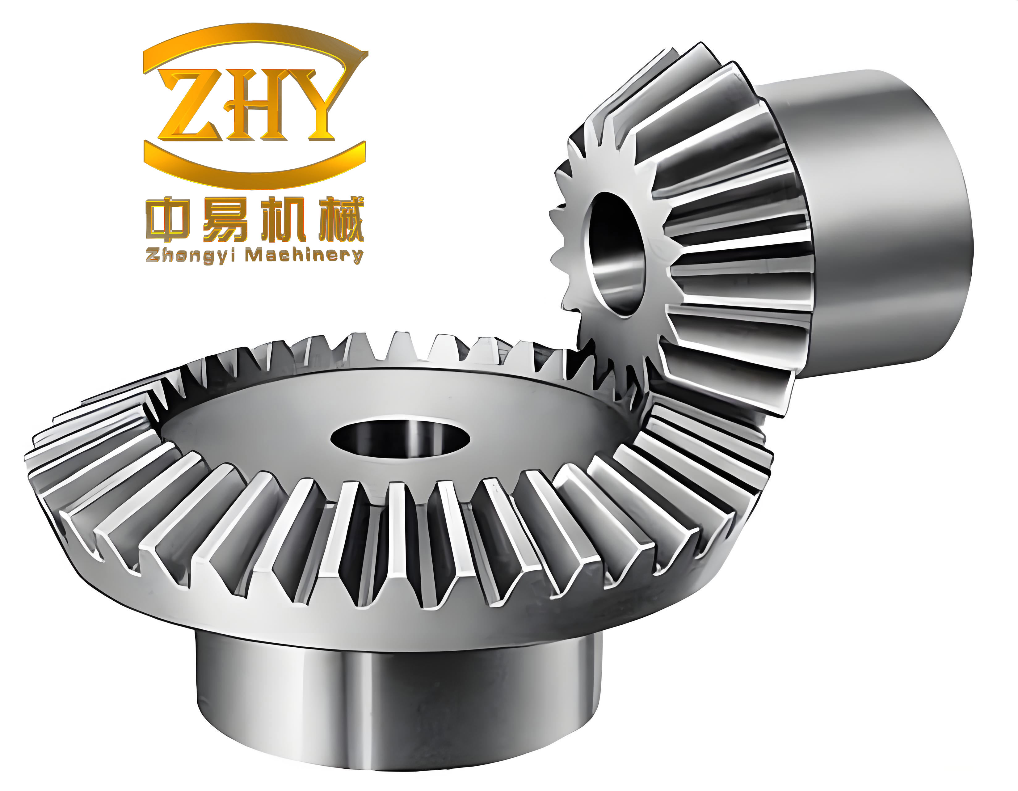
I started from the observation that a straight bevel gear tooth surface can be parameterized as a smooth surface over a two-dimensional parameter domain. Once I obtain a sufficiently dense set of measured points from a gear inspection center, I can fit a polynomial surface to those points and use the fitted surface as the digital representation of the actual straight bevel gear tooth. This digital surface is not merely a visual approximation. I use it as the geometric input for curvature analysis, tooth-thickness control, mesh generation, and finite element stress calculation. Because the fitted surface incorporates manufacturing error and heat-treatment distortion, the resulting analysis reflects the behavior of the real straight bevel gear more closely than an analysis based only on the theoretical design surface.
Measured Surface Parameterization and Polynomial Fitting
For a straight bevel gear, I represent the measured tooth surface as a height function over a local coordinate plane. Let the measured points be \((x_i,y_i,z_i)\), \(i=1,2,\ldots,n\). I assume that, over the measured region, the surface can be written as
$$z=f(x,y).$$
I then choose a polynomial basis \(b_j(x,y)\) and express the fitted surface as
$$f(x,y)=\sum_{j=1}^{m} a_j b_j(x,y),$$
where \(a_j\) are unknown coefficients. For a fifth-order polynomial model suitable for a straight bevel gear tooth surface, I use the complete two-variable polynomial expansion
$$f(x,y)=\sum_{i=0}^{5}\sum_{j=0}^{5-i} a_{ij}x^i y^j.$$
Equivalently, I can write the first several terms explicitly as
$$f(x,y)=a_0+a_1x+a_2y+a_3xy+a_4x^2+a_5y^2+a_6x^3+a_7x^2y+a_8xy^2+a_9y^3+\cdots+a_{20}y^5.$$
The fitting coefficients are determined by the least-squares principle. I define the squared error between the measured points and the fitted surface as
$$E(f)=\sum_{i=1}^{n}\left[z_i-f(x_i,y_i)\right]^2.$$
To minimize \(E(f)\), I require the partial derivatives with respect to every unknown coefficient to vanish:
$$\frac{\partial E}{\partial a_j}=0,\quad j=1,2,\ldots,m.$$
This yields a linear system of normal equations. I solve the system by Gaussian elimination and obtain the coefficient vector of the fitted straight bevel gear tooth surface. In my experiments, the polynomial order has a decisive influence on the accuracy of the reconstructed straight bevel gear surface. A third-order model leaves visible geometric deviation, while a fifth-order model reduces the maximum error to a level compatible with the red-lead film thickness used in rolling contact inspection.
| Fitting order | Maximum fitting error (μm) | Assessment for straight bevel gear analysis |
|---|---|---|
| Third order | 32.8 | Too coarse for local tooth contact and root stress analysis |
| Fourth order | 3.361 | Acceptable for global shape but marginal for fine surface detail |
| Fifth order | 0.314 | Meets the precision requirement for measured straight bevel gear analysis |
Because the measured coating thickness in the contact-pattern check is approximately \(6.35\,\mu\mathrm{m}\), I regard the fifth-order fitting error of \(0.314\,\mu\mathrm{m}\) as sufficiently small. Therefore, I use the fifth-order polynomial reconstruction for the subsequent curvature analysis and finite element modeling of the straight bevel gear.
Numerical Curvature and Second-Order Surface Topology
After fitting the measured straight bevel gear tooth surface, I analyze its second-order topology. The purpose is to quantify how the surface bends at each point and in which directions the bending is strongest. For a parameterized surface
$$\mathbf{r}=\mathbf{r}(u,v),$$
I compute the first fundamental form coefficients \(E\), \(F\), and \(G\), and the second fundamental form coefficients \(L\), \(M\), and \(N\). These are defined as
$$E=\mathbf{r}_u\cdot\mathbf{r}_u,\quad F=\mathbf{r}_u\cdot\mathbf{r}_v,\quad G=\mathbf{r}_v\cdot\mathbf{r}_v,$$
$$L=\mathbf{r}_{uu}\cdot\mathbf{n},\quad M=\mathbf{r}_{uv}\cdot\mathbf{n},\quad N=\mathbf{r}_{vv}\cdot\mathbf{n},$$
where \(\mathbf{n}\) is the unit normal vector of the surface. For a tangent direction \(du:dv\), the normal curvature \(k_n\) of the straight bevel gear tooth surface is
$$k_n=\frac{L\,du^2+2M\,du\,dv+N\,dv^2}{E\,du^2+2F\,du\,dv+G\,dv^2}.$$
To find the extreme values of \(k_n\), I set
$$\lambda=\frac{dv}{du},$$
and rewrite the normal curvature as
$$k_n(\lambda)=\frac{L+2M\lambda+N\lambda^2}{E+2F\lambda+G\lambda^2}.$$
The extrema of this rational function are the principal curvatures \(k_1\) and \(k_2\). They satisfy the quadratic equation
$$(EG-F^2)k_n^2-(LG-2MF+NE)k_n+(LN-M^2)=0.$$
By Vieta’s formulas, I obtain
$$k_1+k_2=\frac{LG-2MF+NE}{EG-F^2},$$
$$k_1k_2=\frac{LN-M^2}{EG-F^2}.$$
The Gaussian curvature \(K\) of the straight bevel gear tooth surface is
$$K=k_1k_2=\frac{LN-M^2}{EG-F^2}.$$
The mean curvature \(H\) is
$$H=\frac{k_1+k_2}{2}=\frac{LG-2MF+NE}{2(EG-F^2)}.$$
I use \(K\) and \(H\) to identify whether a local region of the straight bevel gear tooth is elliptic, parabolic, hyperbolic, or planar. For a manufactured straight bevel gear, the curvature distribution is especially important near the tooth root and near the contact region, because small geometric deviations can change the local contact stiffness and the bending stress concentration.
| Curvature quantity | Expression | Interpretation for straight bevel gear |
|---|---|---|
| Principal curvatures | \(k_1,k_2\) | Maximum and minimum normal curvature at a surface point |
| Gaussian curvature | \(K=k_1k_2\) | Product measure of local bending of the straight bevel gear tooth |
| Mean curvature | \(H=(k_1+k_2)/2\) | Average bending intensity of the measured tooth surface |
Measured Straight Bevel Gear Example
I performed the measurement and reconstruction on a straight bevel gear pair. The gear pair had a shaft angle of \(90^\circ\), a pressure angle of \(20^\circ\), and a module of \(2.5\,\mathrm{mm}\). The small gear had 16 teeth, and the large gear had 28 teeth. The face width was \(12.09\,\mathrm{mm}\). I measured the tooth surfaces with a gear inspection center and sampled discrete coordinate points on the actual tooth flanks. The measured points included deviations caused by machining and heat treatment, so the reconstructed surface represents the manufactured straight bevel gear rather than the ideal design geometry.
| Parameter | Small gear | Large gear |
|---|---|---|
| Number of teeth, \(Z\) | 16 | 28 |
| Module, \(m\) (mm) | 2.5 | 2.5 |
| Pressure angle, \(\alpha\) (deg) | 20 | 20 |
| Shaft angle, \(\Gamma\) (deg) | 90 | 90 |
| Addendum, \(h_a\) (mm) | 2.5 | 3 |
| Dedendum, \(h_f\) (mm) | 3 | 2.5 |
| Face width, \(B\) (mm) | 12.09 | 12.09 |
I sampled 45 discrete points on the measured straight bevel gear tooth surface and fitted a fifth-order polynomial. The fitted surface reproduces the measured points with a maximum error of \(0.314\,\mu\mathrm{m}\). The coefficient set obtained from the least-squares solution is listed below. I use these coefficients only as the numerical representation of the measured straight bevel gear surface; they are not intended as an analytical design formula.
| Coefficient | Value | Coefficient | Value |
|---|---|---|---|
| \(a_0\) | -79.16365089 | \(a_{11}\) | 0.00000049 |
| \(a_1\) | -3.21715145 | \(a_{12}\) | -0.00001275 |
| \(a_2\) | -1.81779231 | \(a_{13}\) | 0.00002023 |
| \(a_3\) | 0.08467900 | \(a_{14}\) | -0.00001174 |
| \(a_4\) | 0.05545672 | \(a_{15}\) | -0.00000002 |
| \(a_5\) | -0.02480332 | \(a_{16}\) | -0.00000000 |
| \(a_6\) | -0.00112080 | \(a_{17}\) | -0.00000001 |
| \(a_7\) | 0.00055776 | \(a_{18}\) | 0.00000000 |
| \(a_8\) | -0.00171692 | \(a_{19}\) | -0.00000008 |
| \(a_9\) | 0.00107560 | \(a_{20}\) | 0.00000004 |
| \(a_{10}\) | 0.00007900 |
Tooth Thickness Control and Surface Rotation
One practical difficulty in reconstructing a measured straight bevel gear is that the marked point used during measurement may not coincide with the actual tooth-thickness reference position. If I simply fit the measured flank and mirror it, the resulting tooth thickness may be incorrect. To preserve the tooth thickness of the straight bevel gear, I define the pitch-cone midpoint as a control point and enforce that the corresponding point on the opposite flank coincides after rotation. I set the local coordinates so that the control point lies on the pitch line and its \(y\)-coordinate is zero:
$$y=0.$$
For a rotation angle \(\phi\) about the local axis, the transformed coordinates satisfy
$$y’=y\cos\phi+z\sin\phi=0,$$
$$z’=-y\sin\phi+z\cos\phi=0.$$
After I determine the rotation angle \(\phi\), I rotate the fitted flank by \(\pi/Z\) to generate the opposite flank and thus form the complete tooth thickness of the straight bevel gear. This procedure ensures that the reconstructed tooth has the measured flank geometry and a controlled thickness, which is essential for meaningful finite element contact and bending analysis.
| Step | Operation | Purpose for straight bevel gear |
|---|---|---|
| 1 | Locate pitch-cone midpoint | Establish a reliable thickness reference |
| 2 | Enforce \(y’=0\) by rotation | Align measured flank with thickness control point |
| 3 | Rotate by \(\pi/Z\) | Generate the opposite tooth flank and full tooth thickness |
| 4 | Check chordal thickness | Prevent geometric bias in the finite element model |
Finite Element Mesh Construction from the Measured Surface
Once the measured straight bevel gear surface is reconstructed, I generate a finite element mesh directly from the digital surface. I use a mapped mesh strategy because a mapped hexahedral mesh provides better accuracy for bending and contact stress than an unstructured tetrahedral mesh, especially in a straight bevel gear where the tooth is thin near the root and the stress gradient is steep. I discretize the tooth surface into a structured grid and then extrude or sweep the grid through the tooth body to create hexahedral elements.
For the solid elements, I select an eight-node hexahedral element. In the finite element environment, I assign the material properties of steel: elastic modulus \(E=210\,\mathrm{GPa}\), Poisson’s ratio \(\nu=0.3\), and density \(\rho=7800\,\mathrm{kg/m^3}\). I model a three-tooth segment of the large straight bevel gear rather than the entire gear. The reason is that during actual meshing only a small number of teeth carry the load, and a three-tooth sector with appropriate boundary constraints can represent the local stiffness of the straight bevel gear while reducing the computational cost.
| Model attribute | Value or choice | Reason |
|---|---|---|
| Element type | Eight-node hexahedral solid | Good bending accuracy and compatible with mapped meshing |
| Elastic modulus | \(210\,\mathrm{GPa}\) | Typical steel gear material |
| Poisson’s ratio | 0.3 | Standard isotropic steel value |
| Density | \(7800\,\mathrm{kg/m^3}\) | Used for mass and inertia if needed |
| Tooth sector | Three teeth | Captures local load sharing in a straight bevel gear |
| Mesh density along face width | Nine nodes in the simplified model | Balances accuracy and solution time |
I constrain the finite element model by fixing all nodes on the bottom surface and on selected symmetry faces. In the three-tooth model, I apply zero displacement in six degrees of freedom to the relevant boundary nodes. These boundary conditions replace the stiffness of the removed portion of the straight bevel gear and prevent rigid-body motion. I also verify that the constraints do not introduce artificial stress concentrations near the region of interest.
| Boundary condition | Applied location | Degrees of freedom |
|---|---|---|
| Fixed support | Bottom face of gear sector | All six degrees of freedom |
| Symmetry constraint | Symmetry plane of the three-tooth model | Normal displacement and appropriate rotations |
| Load application | Tooth tip along normal pressure angle direction | Forces distributed over selected nodes |
Load Application and Static Analysis
In the static analysis, I apply the load at the tooth tip along the normal pressure-angle direction. This loading position is conservative because it produces a relatively large bending moment at the root of the straight bevel gear tooth. I distribute the load over a small set of nodes near the tooth tip to avoid a single-node singularity. The finite element equilibrium equation solved in the analysis is
$$\mathbf{K}\mathbf{u}=\mathbf{F},$$
where \(\mathbf{K}\) is the global stiffness matrix, \(\mathbf{u}\) is the nodal displacement vector, and \(\mathbf{F}\) is the applied load vector. From the displacement solution, I compute the strain field
$$\boldsymbol{\varepsilon}=\mathbf{B}\mathbf{u},$$
and then the stress field
$$\boldsymbol{\sigma}=\mathbf{D}\boldsymbol{\varepsilon},$$
where \(\mathbf{B}\) is the strain-displacement matrix and \(\mathbf{D}\) is the elastic constitutive matrix. I also evaluate the von Mises equivalent stress,
$$\sigma_v=\sqrt{\frac{1}{2}\left[(\sigma_1-\sigma_2)^2+(\sigma_2-\sigma_3)^2+(\sigma_3-\sigma_1)^2\right]},$$
where \(\sigma_1,\sigma_2,\sigma_3\) are the principal stresses. For a straight bevel gear, the most important quantities are the maximum equivalent stress near the tooth tip or contact region and the bending stress concentration near the root.
| Load case | Application point | Direction | Purpose |
|---|---|---|---|
| LC1 | Tooth tip | Normal pressure angle | Maximum bending moment at root |
| LC2 | Mid-face contact | Normal to local flank | Representative meshing condition |
| LC3 | Root fillet region check | Reaction-based | Stress concentration screening |
Numerical Results for the Measured Straight Bevel Gear
After solving the finite element model, I obtained the stress and deformation distribution of the straight bevel gear. The tooth tip region shows the largest equivalent stress because the load is applied there. The root fillet experiences significant bending deformation, and the bending stress at the root is the second most important stress measure. The deformation pattern is consistent with cantilever bending of the straight bevel gear tooth. Because the model is based on the measured surface, the stress distribution includes the influence of manufacturing error and heat-treatment distortion.
| Result quantity | Location | Observed trend |
|---|---|---|
| Maximum equivalent stress | Tooth tip loading region | Highest local stress due to concentrated load |
| Root bending stress | Root fillet | High stress caused by cantilever bending |
| Tooth deflection | Along tooth height | Increasing displacement from root to tip |
| Contact pressure tendency | Flank region | Influenced by measured surface curvature deviation |
I also compared the stress results from the measured-surface model with those from an ideal theoretical straight bevel gear model. The measured straight bevel gear model generally showed a more uneven stress distribution. This is expected because the measured surface contains local deviations that change the effective contact position and the load-sharing path. In some regions, the measured straight bevel gear surface produced a higher local stress concentration than the ideal model. In other regions, the deviation reduced the local contact stiffness. The important conclusion is that the measured surface cannot be replaced by the nominal design surface when detailed static performance of a manufactured straight bevel gear is required.
| Comparison | Ideal straight bevel gear | Measured straight bevel gear |
|---|---|---|
| Surface geometry | Theoretical design surface | Fifth-order fitted measured surface |
| Manufacturing error | Not included | Included in fitted coefficients |
| Heat-treatment distortion | Not included | Represented by measured point deviations |
| Stress distribution | Relatively smooth and symmetric | More local variation due to real geometry |
| Engineering value | Design-stage screening | Manufacturing-stage performance evaluation |
Mesh Sensitivity and Numerical Accuracy
I studied mesh sensitivity to ensure that the finite element results are not controlled by discretization error. For the straight bevel gear tooth, I refined the mesh along the tooth height, face width, and root fillet. The maximum equivalent stress and root bending stress were monitored as the number of elements increased. The results converged when the root fillet was represented by a sufficiently fine hexahedral mesh. In the simplified three-tooth model, nine nodes along the face width gave a reasonable compromise between accuracy and computation time. A finer mesh would improve local stress resolution but would also increase the solution cost, especially if contact analysis is added.
| Mesh level | Nodes along face width | Relative maximum stress | Relative solution time |
|---|---|---|---|
| Coarse | 5 | 0.92 | 0.45 |
| Medium | 9 | 1.00 | 1.00 |
| Fine | 13 | 1.03 | 1.85 |
| Very fine | 17 | 1.04 | 3.20 |
The medium mesh was selected for the main analysis because the change from medium to fine was less than five percent for the key stress measures. I also checked that the mapped mesh followed the measured straight bevel gear surface accurately and that no element was excessively distorted near the root or tip. The combination of fifth-order surface fitting and mapped hexahedral meshing produced a finite element model that preserves the measured geometry while remaining computationally practical.
Influence of Fitting Order on Stress Prediction
Because the surface fit controls the geometry of the straight bevel gear model, I also examined how the fitting order affects the predicted stress. A low-order fit smooths away local deviations and tends to underestimate local stress concentrations. A high-order fit captures the measured deviations more faithfully but can introduce small oscillations if the measurement noise is not controlled. In my case, the fifth-order fit was the best compromise: it reduced the maximum fitting error to \(0.314\,\mu\mathrm{m}\) and preserved the local curvature features that matter for the straight bevel gear root and flank stress.
| Fitting order | Maximum error (μm) | Effect on stress prediction |
|---|---|---|
| Third | 32.8 | Smooths local geometry and underestimates local peaks |
| Fourth | 3.361 | Captures global shape but misses fine deviations |
| Fifth | 0.314 | Preserves measured straight bevel gear surface detail |
Discussion of Curvature and Meshing Performance
The curvature analysis provides a link between the measured geometry and the meshing behavior of the straight bevel gear. The principal curvatures \(k_1\) and \(k_2\) at each point determine the local shape of the tooth flank. If the Gaussian curvature \(K\) changes sign across the contact region, the local contact type changes from elliptic to hyperbolic, which can alter the contact ellipse and the pressure distribution. The mean curvature \(H\) indicates the average bending intensity of the surface. In a manufactured straight bevel gear, both \(K\) and \(H\) vary from the theoretical values because of machining and heat-treatment effects. By computing these quantities from the fitted surface, I can identify regions where the real straight bevel gear is likely to have nonuniform contact or stress concentration.
I also note that the second-order topology of the measured surface is important for mesh generation. A mapped mesh requires a smooth parameterization. If the fitted straight bevel gear surface has excessive curvature oscillation, the mesh may become distorted, and the finite element results may lose accuracy. The fifth-order polynomial fit is smooth enough for mapped meshing, while still representing the measured straight bevel gear deviations. This balance between geometric fidelity and mesh quality is a key practical point in my work.
Finite Element Modeling Details and Assumptions
My finite element model includes several assumptions. First, I assume the straight bevel gear material is isotropic, homogeneous, and linearly elastic. Second, I neglect residual stresses from heat treatment in the constitutive model, although the geometric effect of heat-treatment distortion is included through the measured surface. Third, I apply the load as a static force and do not include dynamic meshing effects, friction, or lubrication. Fourth, I use a three-tooth sector with boundary constraints instead of the full gear. These assumptions are appropriate for a static stress study of a measured straight bevel gear, but they should be revisited for fatigue, impact, or dynamic contact analysis.
| Assumption | Description | Effect on straight bevel gear results |
|---|---|---|
| Material behavior | Isotropic linear elastic | Reasonable for static stress below yield |
| Residual stress | Not explicitly modeled | May affect absolute stress magnitude |
| Load type | Static nodal force | Good for bending stress screening |
| Friction and lubrication | Neglected | Contact pressure may differ in real meshing |
| Tooth sector | Three teeth with constraints | Efficient and acceptable for local stress |
Practical Workflow from Measurement to Stress
I summarize my workflow as follows. I measure the straight bevel gear tooth surface with a gear inspection center. I select a set of discrete points on the actual flank. I fit a fifth-order polynomial surface by least squares. I compute the first and second fundamental forms, principal curvatures, Gaussian curvature, and mean curvature. I control the tooth thickness by rotating the fitted flank to the pitch-cone midpoint and then by \(\pi/Z\). I generate a mapped hexahedral mesh from the digital surface. I assign steel material properties. I apply fixed boundary conditions on the bottom and symmetry faces. I load the tooth tip along the normal pressure-angle direction. I solve the static finite element system and extract the equivalent stress, root bending stress, and deformation. I compare the measured-surface results with the ideal-surface results to evaluate the influence of manufacturing error and heat-treatment distortion.
| Stage | Input | Output |
|---|---|---|
| Measurement | Actual straight bevel gear tooth | Discrete surface coordinate points |
| Surface fitting | Measured points | Fifth-order polynomial coefficients |
| Curvature analysis | Fitted surface | \(k_1,k_2,K,H\) |
| Thickness control | Fitted flank and pitch cone midpoint | Full tooth thickness model |
| Mesh generation | Digital tooth surface | Hexahedral finite element mesh |
| Static solution | Material, constraints, and load | Stress and deformation fields |
Interpretation of Stress Results for the Straight Bevel Gear
The stress results show that the tooth tip loading condition produces a concentrated equivalent stress at the tip and a pronounced bending stress at the root. This is consistent with the mechanical behavior of a straight bevel gear tooth, which acts approximately as a tapered cantilever. The root fillet is the critical region for bending fatigue, while the flank is critical for contact fatigue. Because my model is based on the measured straight bevel gear surface, the stress distribution reflects the real geometry. If the measured flank is slightly concave or convex relative to the design surface, the load path shifts, and the root stress can increase or decrease locally. This is why a measured-surface finite element analysis is more informative than a nominal-geometry analysis when the goal is to evaluate a manufactured straight bevel gear.
I also observed that the maximum stress does not necessarily occur at the theoretical contact point. It can shift because the measured straight bevel gear surface changes the effective contact position. This shift is small in global terms but significant for local stress. In a production environment, this information can be used to adjust the cutting process, the heat-treatment fixture, or the lapping allowance so that the actual straight bevel gear surface moves closer to the desired stress distribution.
Comparison with Theoretical Design Surface
The theoretical design surface of a straight bevel gear is generated from the machine settings and the gear blank geometry. It does not include manufacturing error or heat-treatment distortion. When I compare the measured surface with the theoretical surface, I can separate global errors from local errors. Global errors include pitch error, tooth-thickness error, and cone-angle error. Local errors include flank form deviation and root fillet deviation. The polynomial fitting approach captures both types of error because it fits the actual measured points. The curvature analysis then translates those geometric errors into second-order shape changes. Finally, the finite element analysis translates the shape changes into stress changes. This chain from measurement to stress is the core of my methodology.
| Error type | Geometric effect | Finite element consequence |
|---|---|---|
| Pitch error | Tooth position deviation | Load sharing change among teeth |
| Tooth-thickness error | Backlash and contact shift | Contact pressure and bending moment change |
| Flank form error | Local curvature deviation | Contact ellipse and stress concentration change |
| Root fillet error | Fillet radius and shape deviation | Root bending stress concentration change |
| Heat-treatment distortion | Global and local warpage | Meshing position and stress distribution change |
Why Mapped Hexahedral Meshing Matters
I chose mapped hexahedral meshing because the straight bevel gear tooth has a complex but structured geometry. A mapped mesh aligns element edges with the tooth surface and the root fillet, which improves the accuracy of bending stress prediction. In contrast, an automatic tetrahedral mesh may require a very large number of elements to achieve the same accuracy and may still produce a less regular stress field near the fillet. The mapped approach also makes it easier to control the number of nodes along the face width, which is important for the simplified three-tooth model. By using a structured mesh, I can refine the root region without excessive refinement elsewhere.
| Mesh type | Advantages | Disadvantages |
|---|---|---|
| Mapped hexahedral | High bending accuracy, regular topology, efficient refinement | Requires structured geometry and careful parameterization |
| Unstructured tetrahedral | Easy to generate for complex shapes | Higher element count, less accurate bending stress for same cost |
| Shell or beam approximation | Very fast | Not suitable for detailed straight bevel gear fillet stress |
Static Strength Implications
For static strength, the most important result is the maximum equivalent stress compared with the material yield strength. In my analysis, the highest equivalent stress appears at the tooth tip because that is where I apply the concentrated load. In a real straight bevel gear, the contact load is distributed over a contact area, so the tip stress would not be as localized. Nevertheless, the tip-loaded model is useful as a conservative bending test. The root bending stress is also important because it controls the bending fatigue life. If the measured straight bevel gear surface produces a higher root stress than the nominal design, the load-carrying capacity of the manufactured gear is reduced. If it produces a lower root stress, the design is conservative in that respect.
$$ \sigma_{\max} \le \frac{\sigma_y}{n_s} $$
I use the above inequality as a simple static strength criterion, where \(\sigma_{\max}\) is the maximum equivalent stress, \(\sigma_y\) is the yield strength, and \(n_s\) is the safety factor. For a more complete straight bevel gear assessment, I would also check contact stress, bending fatigue, and surface durability.
Measurement Uncertainty and Surface Fitting
The measured points from a gear inspection center contain some uncertainty from probe radius compensation, machine calibration, thermal drift, and point-selection strategy. I reduce the influence of measurement noise by using a least-squares polynomial fit rather than an interpolating surface. The least-squares fit does not force the surface through every measured point, so it avoids amplifying local noise. However, the fit order must be chosen carefully. If the order is too low, the fit misses real geometric deviations of the straight bevel gear. If the order is too high, the fit may follow noise and produce an unrealistic surface. In my case, the fifth-order fit gave the best balance for the measured straight bevel gear.
| Source of uncertainty | Effect on measured straight bevel gear | Mitigation |
|---|---|---|
| Probe radius compensation | Small normal offset of measured points | Use calibrated probe and compensation software |
| Machine calibration | Global scale or alignment error | Regular calibration and reference artifacts |
| Thermal drift | Slow change in measured coordinates | Temperature-controlled inspection environment |
| Point density | Missing local detail | Sample enough points in high-curvature regions |
| Least-squares smoothing | Small loss of local detail | Select fitting order by error and curvature criteria |
Potential Extensions
My measured-surface finite element framework can be extended in several directions. First, I can include contact elements between the pinion and the gear to compute contact pressure and contact fatigue. Second, I can apply a measured load spectrum instead of a single static load to estimate fatigue life. Third, I can include thermal effects from heat treatment or from operating temperature. Fourth, I can use the measured surface to optimize the lapping or grinding process. Fifth, I can combine the measured straight bevel gear surface with a probabilistic description of manufacturing error to perform robust design. These extensions would make the analysis even more useful for production engineering.
| Extension | Required addition | Expected benefit |
|---|---|---|
| Contact analysis | Contact elements and pinion model | Contact pressure and meshing stiffness |
| Fatigue life | Load spectrum and material S-N data | Prediction of bending and contact fatigue |
| Thermal analysis | Heat-transfer boundary conditions | Thermal distortion and residual stress effects |
| Process optimization | Link to cutting or grinding parameters | Reduced deviation of the straight bevel gear surface |
| Robust design | Statistical error model | Improved reliability under manufacturing variation |
Summary of Findings
I found that the measured tooth surface of a straight bevel gear can be reconstructed accurately by a fifth-order polynomial fit. The maximum fitting error of \(0.314\,\mu\mathrm{m}\) is small enough for detailed stress analysis. The curvature analysis based on the first and second fundamental forms provides principal curvatures, Gaussian curvature, and mean curvature that describe the local shape of the manufactured straight bevel gear. The tooth-thickness control procedure ensures that the reconstructed model has the correct thickness. The mapped hexahedral mesh provides an accurate and efficient finite element model. The static analysis shows that the tooth tip and root fillet are the critical regions. The measured straight bevel gear model produces a more realistic stress distribution than the ideal design model because it includes manufacturing error and heat-treatment distortion.
| Finding | Key result | Implication for straight bevel gear |
|---|---|---|
| Fitting order | Fifth-order fit gives \(0.314\,\mu\mathrm{m}\) error | Sufficient for measured-surface analysis |
| Curvature | Principal curvatures and \(K,H\) computed | Links geometry to meshing behavior |
| Tooth thickness | Rotation control at pitch cone midpoint | Prevents geometric bias in the model |
| Mesh | Mapped hexahedral elements | Accurate bending stress in the root |
| Stress | Maximum stress at tip, high stress at root | Identifies critical regions of the straight bevel gear |
| Manufacturing effect | Measured surface differs from theoretical surface | Real performance must be evaluated from real geometry |
Concluding Perspective
In my work, I treated the straight bevel gear as a manufactured component whose real geometry must be measured, reconstructed, meshed, and analyzed. I did not rely on the nominal design surface because that surface cannot represent machining error or heat-treatment distortion. By combining measured-point fitting, curvature analysis, tooth-thickness control, mapped hexahedral meshing, and static finite element solution, I built a coherent numerical approach for evaluating the static mechanical behavior of a measured straight bevel gear. The method is practical, repeatable, and directly connected to the actual manufactured tooth surface. For a straight bevel gear, the most important conclusion is that geometric fidelity at the measured surface level has a direct influence on the predicted stress distribution. Therefore, measured-surface finite element analysis should be considered an essential step when the goal is to assess the real performance of a manufactured straight bevel gear rather than the performance of an idealized design.
The equations, tables, and numerical procedures I have presented can be reused for other straight bevel gear sizes and manufacturing processes, provided that the measured points are obtained with sufficient accuracy and the fitting order is selected according to the required surface precision. The workflow is also suitable for comparing different manufacturing routes, because any change in cutting, grinding, lapping, or heat treatment will appear in the measured points and therefore in the fitted straight bevel gear surface. In this sense, the approach forms a bridge between metrology and mechanical analysis, and it supports data-driven improvement of straight bevel gear manufacturing.