
In my research, I investigate the nonlinear dynamic behavior of a helical gear transmission system when the flash temperature generated at the meshing tooth surfaces is taken into account. The helical gear pair operates under high-speed and high-power conditions, such as those found in railway traction gearboxes. The temperature rise at the contact interface changes the tooth profile deformation, the lubricant film properties, the friction coefficient, and the time-varying meshing stiffness. These changes, in turn, alter the dynamic response of the entire helical gear system. I combine Hertzian elastic contact theory, elastohydrodynamic lubrication theory, and nonlinear dynamics to build a comprehensive model. The main goal is to quantify how flash temperature affects oil film stiffness, friction excitation, and the bifurcation characteristics of the helical gear transmission.
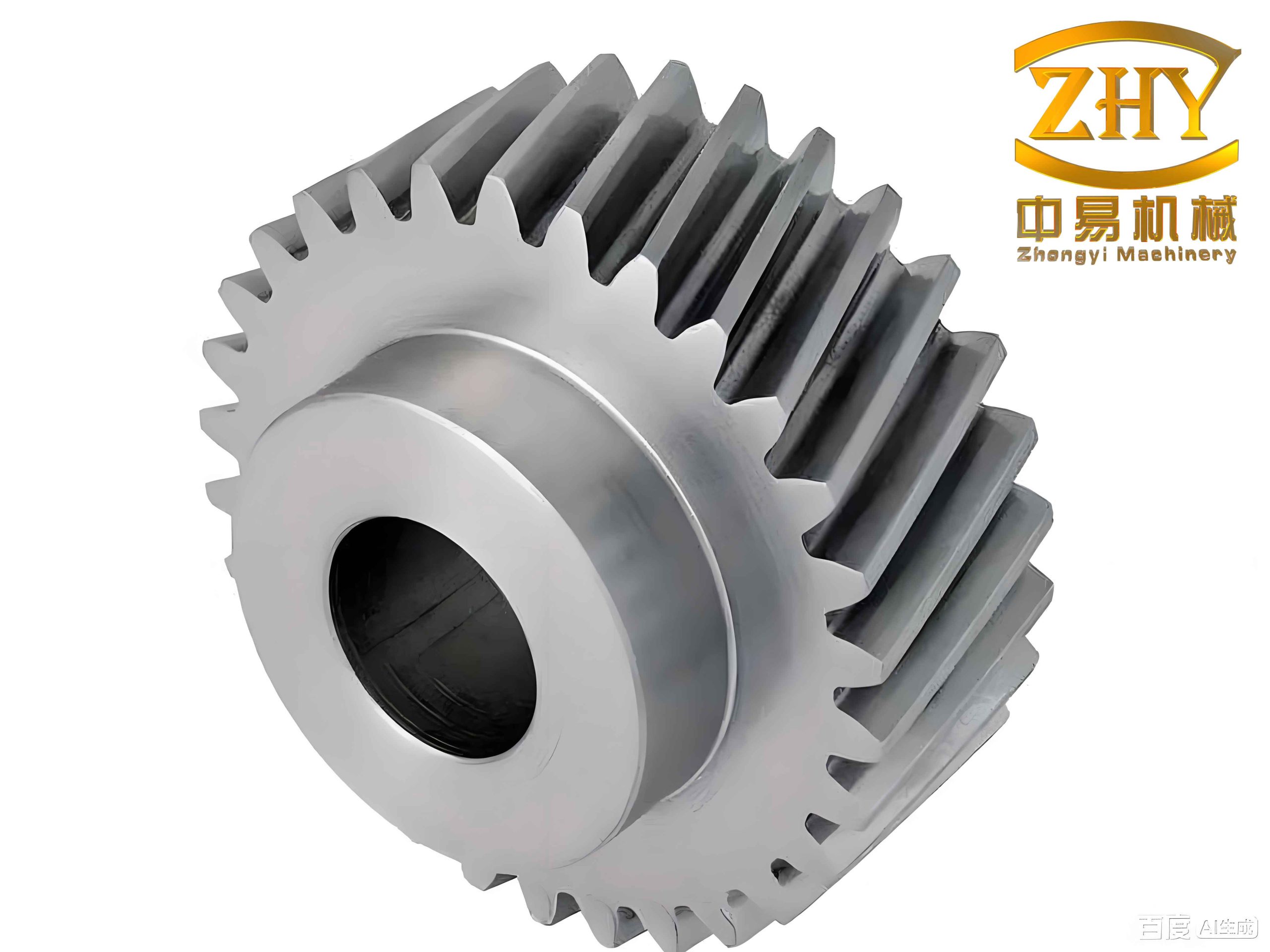
The helical gear is widely used in high-speed drivetrains because its gradual tooth engagement produces smoother transmission than spur gears. However, the sliding between the meshing flanks inevitably generates heat. The heat cannot dissipate instantaneously, so a local temperature spike, known as the flash temperature, appears. This flash temperature reduces the lubricant viscosity, decreases the film thickness, and modifies the contact stiffness. My work addresses three questions: how the contact line length and load sharing vary along the line of action, how the line-contact and point-contact thermal elastohydrodynamic lubrication (TEHL) models predict film thickness, pressure, and flash temperature, and how the flash-temperature-dependent stiffness and friction alter the nonlinear dynamics of the helical gear system.
1. Meshing Process and Contact Line Length of the Helical Gear
The helical gear pair I study has the basic parameters listed in Table 1. The transverse module, transverse pressure angle, and base helix angle are calculated from the normal parameters. These values are used throughout my contact and dynamic analyses.
| Parameter | Symbol | Driving Gear | Driven Gear |
|---|---|---|---|
| Number of teeth | z | 29 | 69 |
| Face width (mm) | B | 75 | 70 |
| Normal module (mm) | m_n | 7 | 7 |
| Normal pressure angle (deg) | alpha_n | 26 | 26 |
| Helix angle (deg) | beta | 20 | 20 |
| Addendum coefficient | h_a^* | 1 | 1 |
| Clearance coefficient | c^* | 0.25 | 0.25 |
| Load torque (N m) | T | 100 | 100 |
The transverse module is $$m_t = \frac{m_n}{\cos\beta}$$ and the transverse pressure angle is $$\alpha_t = \arctan\left(\frac{\tan\alpha_n}{\cos\beta}\right).$$ The base helix angle is $$\beta_b = \arctan\left(\tan\beta \cos\alpha_t\right).$$ For a helical gear, the total contact ratio is the sum of the transverse contact ratio and the overlap contact ratio. The transverse contact ratio is $$\varepsilon_\alpha = \frac{z_1(\tan\alpha_{at1}-\tan\alpha_t’) + z_2(\tan\alpha_{at2}-\tan\alpha_t’)}{2\pi},$$ and the overlap contact ratio is $$\varepsilon_\beta = \frac{B \sin\beta}{\pi m_n}.$$ The total contact ratio is $$\varepsilon = \varepsilon_\alpha + \varepsilon_\beta.$$ Because the helical gear has inclined teeth, the contact line length changes continuously rather than abruptly. I divide one meshing period into five stages according to the number of simultaneously meshing tooth pairs. The contact line length for a single tooth pair can be written as a piecewise function. When the transverse contact ratio is smaller than the overlap contact ratio, the length is $$L(\theta) = \begin{cases} \frac{B}{\sin\beta_b} & \theta_1 \le \theta \le \theta_2 \\ \frac{B}{\sin\beta_b} \frac{\theta_5-\theta}{\theta_5-\theta_4} & \theta_2 \le \theta \le \theta_5 \\ 0 & \theta_5 \le \theta \le \theta_7 \end{cases}$$ where the angles define the boundaries of the meshing zones. The total contact line length at any instant is the sum over all meshing tooth pairs: $$L_{\text{total}}(\theta) = \sum_{i=1}^{n} L_i(\theta).$$ I also compute the load sharing coefficient as $$\lambda(\theta) = \frac{L(\theta)}{L_{\text{total}}(\theta)}.$$ The contact line length and load sharing coefficient vary periodically, and their abrupt changes at the transitions between two-tooth and three-tooth contact are the main sources of internal excitation in the helical gear system.
| Stage | Number of meshing pairs | Contact line behavior |
|---|---|---|
| Entry | 2 or 3 | Short contact line, rapid increase |
| Transition 2-3 | 2 to 3 | Step increase in total length |
| Full contact | 3 | Maximum total length |
| Transition 3-2 | 3 to 2 | Step decrease in total length |
| Exit | 2 | Contact line decreases to zero |
The influence of module, tooth number ratio, pressure angle, and helix angle on the contact line length is summarized in Table 2. Increasing the module enlarges the amplitude of the contact line length variation and narrows the stable two-tooth contact zone. The tooth number ratio mainly shifts the curve downward without changing its shape. A larger pressure angle widens the two-tooth zone and narrows the three-tooth zone. A smaller helix angle makes the curve steeper and closer to that of a spur gear, which increases the impact between teeth. Therefore, proper parameter selection is critical for a stable helical gear drive.
2. Relative Sliding and Entrainment Velocity
On the line of action, any meshing point K has coordinates relative to the pitch point. The radii of curvature of the driving and driven gears are $$R_1 = r_1 \sin\alpha_n – x_k, \quad R_2 = r_2 \sin\alpha_n + x_k.$$ The equivalent radius is $$R = \frac{R_1 R_2}{R_1 + R_2}.$$ The tangential velocities of the two tooth surfaces at point K are $$u_1 = \omega_1 R_1, \quad u_2 = \omega_2 R_2.$$ The relative sliding velocity is $$u_s = u_1 – u_2,$$ and the entrainment velocity is $$u_e = \frac{u_1 + u_2}{2}.$$ The slide-to-roll ratio is $$SR = \frac{u_s}{u_e}.$$ I computed these quantities for rotational speeds from 500 r/min to 2000 r/min. The relative sliding velocity changes sign along the line of action, being zero at the pitch point. Its absolute value first decreases and then increases. The entrainment velocity increases from the engaging point to the disengaging point. The slide-to-roll ratio is independent of speed and follows the same trend as the relative sliding velocity. These velocities are essential inputs for the thermal elastohydrodynamic lubrication analysis of the helical gear.
| Rotational speed (r/min) | Entrainment velocity range (m/s) | Relative sliding velocity range (m/s) | Slide-to-roll ratio range |
|---|---|---|---|
| 500 | 0.65 – 1.30 | -1.10 – 1.10 | -1.00 – 1.00 |
| 1000 | 1.30 – 2.60 | -2.20 – 2.20 | -1.00 – 1.00 |
| 1500 | 1.95 – 3.90 | -3.30 – 3.30 | -1.00 – 1.00 |
| 2000 | 2.60 – 5.20 | -4.40 – 4.40 | -1.00 – 1.00 |
3. Line-Contact Thermal Elastohydrodynamic Lubrication Model
I model the contact between two helical gear teeth as a line contact between an equivalent elastic cylinder and a rigid plane. The Hertzian contact half-width is $$a = \sqrt{\frac{8 w R}{\pi E’}},$$ where the equivalent elastic modulus is $$\frac{1}{E’} = \frac{1}{2}\left(\frac{1-\nu_1^2}{E_1} + \frac{1-\nu_2^2}{E_2}\right).$$ The Hertzian pressure distribution is $$p_H(x) = p_{\max} \sqrt{1 – \frac{x^2}{a^2}},$$ with the maximum pressure $$p_{\max} = \frac{2w}{\pi a} = \sqrt{\frac{w E’}{2\pi R}}.$$ The elastic deformation of the surfaces is $$h_e(x) = -\frac{2}{\pi E’} \int_{x_0}^{x_e} p(s) \ln(s-x)^2 ds + c.$$ The Reynolds equation for line contact is $$\frac{d}{dx}\left(\frac{\rho h^3}{12\eta}\frac{dp}{dx}\right) = u_e \frac{d(\rho h)}{dx}.$$ The energy equation is $$\rho c_p u \frac{\partial T}{\partial x} – \frac{\partial}{\partial z}\left(K \frac{\partial T}{\partial z}\right) = \eta \left(\frac{\partial u}{\partial z}\right)^2.$$ The film thickness equation is $$h(x) = h_0 + \frac{x^2}{2R} + h_e(x).$$ The viscosity-pressure-temperature relationship is given by the Roelands equation: $$\eta = \eta_0 \exp\left\{(\ln\eta_0 + 9.67)\left[-1 + (1 + 5.1 \times 10^{-9} p)^{0.68} \left(\frac{T-138}{T_0-138}\right)^{-1.1}\right]\right\}.$$ The density-pressure-temperature equation is $$\rho = \rho_0 \left[1 + \frac{0.6 p}{1 + 1.7 p} – 0.00065 (T – T_0)\right].$$ The load balance equation is $$\int_{x_0}^{x_e} p(x) dx = w.$$ I nondimensionalize these equations using $$X = \frac{x}{a}, \quad P = \frac{p}{p_H}, \quad H = \frac{h R}{a^2}, \quad \bar{\eta} = \frac{\eta}{\eta_0}, \quad \bar{\rho} = \frac{\rho}{\rho_0}, \quad \bar{T} = \frac{T}{T_0}.$$ The dimensionless Reynolds equation becomes $$\frac{d}{dX}\left(\bar{\rho} H^3 \bar{\eta}^{-1} \frac{dP}{dX}\right) – \lambda \frac{d(\bar{\rho} H)}{dX} = 0,$$ where $$\lambda = \frac{12 u_e \eta_0 R^2}{a^3 p_H}.$$ I solve the coupled equations using finite difference discretization and iterative methods. The pressure distribution is obtained from the Reynolds equation, the film thickness from the elastic deformation integral, and the temperature from the energy equation. The viscosity and density are updated with the new temperature and pressure until convergence.
| Parameter | Value | Unit |
|---|---|---|
| Ambient temperature | 303 | K |
| Initial viscosity | 0.08 | Pa s |
| Pressure-viscosity coefficient | 2.2e-8 | Pa^{-1} |
| Temperature-viscosity coefficient | 0.04 | K^{-1} |
| Equivalent elastic modulus | 2.2e11 | Pa |
| Thermal conductivity | 0.14 | W/(m K) |
| Specific heat | 2000 | J/(kg K) |
The simulation results show that as the rotational speed increases, the film thickness increases, the minimum film position moves away from the exit, and the second pressure peak grows and moves toward the inlet. The flash temperature at the center of the contact reaches a maximum and increases with speed. When the transmitted power increases, the load increases, the film thickness and the second pressure peak decrease, and the flash temperature rises. The lubricant viscosity decreases sharply with temperature up to about 350 K and then levels off. A lower viscosity reduces the film thickness, lowers the second pressure peak, and moves it toward the exit until it disappears. These trends are consistent with classical elastohydrodynamic lubrication theory and highlight the strong coupling between flash temperature and film behavior in the helical gear contact.
4. Point-Contact Thermal Elastohydrodynamic Lubrication at Engagement and Disengagement
At the points where the number of meshing tooth pairs changes, the contact condition becomes closer to point contact. I developed a point-contact TEHL model to study the oil film and flash temperature at these critical locations. The Reynolds equation for point contact is $$\frac{\partial}{\partial x}\left(\frac{\rho h^3}{12\eta}\frac{\partial p}{\partial x}\right) + \frac{\partial}{\partial y}\left(\frac{\rho h^3}{12\eta}\frac{\partial p}{\partial y}\right) = u_e \frac{\partial(\rho h)}{\partial x}.$$ The energy equation is $$\rho c_p \left(u \frac{\partial T}{\partial x} + v \frac{\partial T}{\partial y}\right) = K \left(\frac{\partial^2 T}{\partial x^2} + \frac{\partial^2 T}{\partial y^2} + \frac{\partial^2 T}{\partial z^2}\right) + \eta \left[\left(\frac{\partial u}{\partial z}\right)^2 + \left(\frac{\partial v}{\partial z}\right)^2\right].$$ The film thickness equation is $$h(x,y) = h_0 + \frac{x^2}{2R_x} + \frac{y^2}{2R_y} + h_e(x,y),$$ where the elastic deformation is $$h_e(x,y) = \frac{2}{\pi E’} \iint_\Omega \frac{p(x’,y’)}{\sqrt{(x-x’)^2 + (y-y’)^2}} dx’ dy’.$$ The viscosity and density equations are the same as in the line-contact model. The load balance equation is $$\iint_\Omega p(x,y) dx dy = F.$$ I solve these equations using the multigrid method with Gauss-Seidel and Jacobi dipole iterations. The computational flow starts with an initial pressure and temperature distribution, calculates the film thickness and viscosity, solves the Reynolds equation for a new pressure, updates the energy equation for temperature, and repeats until convergence. I analyze two key points: the 2-3 transition (where two tooth pairs become three) and the 3-2 transition (where three tooth pairs become two). The operating parameters are given in Table 4.
| Parameter | Symbol | 2-3 point | 3-2 point |
|---|---|---|---|
| Line load (N) | w | 471.6 | 531.0 |
| Equivalent radius (m) | R | 0.0395 | 0.0279 |
| Relative sliding velocity (m/s) | u_s | 1.1362 | 1.1992 |
| Entrainment velocity (m/s) | u_e | 3.1268 | 2.6502 |
| Slide-to-roll ratio | SR | 0.3634 | 0.4525 |
The point-contact results show that the oil film pressure is columnar and increases sharply in the contact region. The film thickness distribution is basin-shaped with a central depression, and the minimum film occurs at the edge of the contact zone. The flash temperature distribution follows the pressure distribution. At the 3-2 point, the maximum oil film pressure reaches 0.8231 GPa, the minimum film thickness is 0.1068 micrometers, and the flash temperature rise is 59.9379 K. At the 2-3 point, the maximum pressure is 0.6349 GPa, the minimum film thickness is 0.2039 micrometers, and the flash temperature rise is 32.5466 K. The flash temperature at the point contact is much higher than that in the line contact. The load largely determines the maximum oil film pressure, while the relative sliding velocity determines the minimum film thickness. The flash temperature reaches its maximum at the disengagement point, which explains why tooth tip and root failures such as scuffing and wear are more likely to occur there.
| Quantity | Symbol | 3-2 point | 2-3 point |
|---|---|---|---|
| Maximum oil film pressure (GPa) | p_max | 0.8231 | 0.6349 |
| Minimum oil film thickness (μm) | h_min | 0.1068 | 0.2039 |
| Flash temperature rise (K) | ΔT | 59.9379 | 32.5466 |
5. Dynamic Excitations in the Helical Gear System
The internal excitations of the helical gear system include backlash, static transmission error, time-varying meshing stiffness, meshing damping, and tooth friction. I model the backlash function as $$f(p) = \begin{cases} p – b & p > b \\ 0 & |p| \le b \\ p + b & p < -b \end{cases}$$ where p is the relative displacement and b is half the backlash. The static transmission error is expanded in a Fourier series: $$e(t) = e_0 + \sum_{j=1}^{\infty} e_j \cos(j \omega_e t + \phi_j).$$ In most dynamic studies, only the first harmonic is retained: $$e(t) = e_0 + e_1 \cos(\omega_e t).$$ The time-varying meshing stiffness of a single tooth pair is calculated from an empirical formula: $$K_i(s) = k_p \exp\left[ C_a \frac{s – s_p}{p_{bt}} \right]^{2.25},$$ where s is the position along the line of action, k_p is the stiffness at the pitch point, and C_a is a correction coefficient. The total meshing stiffness is the sum over all meshing pairs: $$K(s) = \sum_{i=1}^{n} K_i(s).$$ I incorporate the flash temperature effect through the oil film stiffness. The oil film stiffness is $$k_{\text{oil}} = \frac{L}{n} \sum_{i=1}^{n} \frac{p(x_i)}{h(x_i)}.$$ The time-varying meshing stiffness with flash temperature is then obtained by combining the tooth stiffness and the oil film stiffness. The result shows that the flash temperature reduces the overall meshing stiffness but does not change its periodic trend. I fit the stiffness curve with an eight-order Fourier series: $$k(t) = \frac{a_0}{2} + \sum_{n=1}^{8} \left[ a_n \cos(n \omega t) + b_n \sin(n \omega t) \right].$$ The fitting coefficients are given in Table 5. The meshing damping is calculated from the empirical formula $$c_m = 2 \xi_g \sqrt{\frac{k_m r_{pb}^2 r_{gb}^2 I_p I_g}{r_{pb}^2 I_p + r_{gb}^2 I_g}},$$ where xi_g is the damping ratio. The friction coefficient is computed from an empirical formula that depends on viscosity, surface roughness, equivalent radius, and maximum Hertzian pressure. The friction force is $$f_i(t) = \mu_i(t) w,$$ and the total friction force is $$F_f(t) = \sum_{i=1}^{n} f_i(t).$$ The friction torque on the driving and driven gears is $$T_{fp}(t) = \sum_{i=1}^{n} f_i(t) L_{pi}(t), \quad T_{fg}(t) = \sum_{i=1}^{n} f_i(t) L_{gi}(t).$$ The friction coefficient is zero at the pitch point and has peaks near the tooth tip and root. I fit the friction torques with a fifth-order Fourier series to obtain smooth expressions for the dynamic equations.
| Order n | a_n (driving) | b_n (driving) | a_n (driven) | b_n (driven) |
|---|---|---|---|---|
| 0 | 0.00226 | 0.00000 | -0.03181 | 0.00000 |
| 1 | -0.02149 | 0.01416 | 0.03234 | -0.05978 |
| 2 | 0.01596 | 0.00688 | -0.04116 | -0.02195 |
| 3 | 0.00314 | 0.01854 | -0.01299 | -0.04686 |
| 4 | -0.00171 | 0.00148 | 0.00028 | -0.00743 |
| 5 | 0.00905 | 0.00210 | -0.02283 | -0.00699 |
6. Nonlinear Dynamic Model of the Helical Gear Transmission
I use the lumped-mass method to build a five-degree-of-freedom dynamic model of the helical gear pair. The model includes the transverse displacements of the driving and driven gears in the y and z directions, and the rotational displacement. The equations of motion without flash temperature are $$I_p \ddot{\theta}_p + r_{pb} F_y = T_p,$$ $$I_g \ddot{\theta}_g – r_{gb} F_y = -T_g,$$ $$m_p \ddot{y}_p + c_{py} \dot{y}_p + k_{py} y_p = F_y,$$ $$m_g \ddot{y}_g + c_{gy} \dot{y}_g + k_{gy} y_g = -F_y,$$ $$m_p \ddot{z}_p + c_{pz} \dot{z}_p + k_{pz} z_p = F_z,$$ $$m_g \ddot{z}_g + c_{gz} \dot{z}_g + k_{gz} z_g = -F_z.$$ The dynamic meshing force is $$F_y = k_m f(p) + c_m \dot{p},$$ and the axial force is $$F_z = F_y \tan\beta.$$ The relative displacement is $$p = y_p – y_g – z_p \tan\beta + z_g \tan\beta – r_{pb} \theta_p + r_{gb} \theta_g – e(t).$$ Combining the torsional equations yields the relative dynamic equation: $$m_e \ddot{p} + c_m \dot{p} + k_m f(p) = F_{pm} + F_e(t),$$ where the equivalent mass is $$m_e = \frac{I_p I_g}{I_p r_{gb}^2 + I_g r_{pb}^2}.$$ The internal excitation is $$F_e(t) = m_e e_1 \omega_e^2 \cos(\omega_e t).$$ When flash temperature is considered, the friction torque terms appear: $$I_p \ddot{\theta}_p + r_{pb} F_y – T_{fp} = T_p,$$ $$I_g \ddot{\theta}_g – r_{gb} F_y + T_{fg} = -T_g.$$ The relative dynamic equation becomes $$m_e \ddot{p} + c_m \dot{p} + k_T f(p) = F_{pm} + F_e(t) + G_p – G_g,$$ where $$G_p = \frac{m_e r_{pb} T_{fp}}{I_p}, \quad G_g = \frac{m_e r_{gb} T_{fg}}{I_g}.$$ I nondimensionalize the equations using the natural frequency $$\omega_n = \sqrt{k_m / m_e},$$ the dimensionless time $$\tau = \omega_n t,$$ and the dimensionless frequency $$\Omega = \omega_e / \omega_n.$$ The state-space equations are solved using the fourth-fifth order Runge-Kutta method. The bifurcation parameter is the dimensionless meshing frequency. I compare the system with and without flash temperature by examining bifurcation diagrams, phase portraits, Poincare sections, and time histories.
| Parameter | Symbol | Value |
|---|---|---|
| Support stiffness (y direction) | k_{py}, k_{gy} | 1.2 |
| Support stiffness (z direction) | k_{pz}, k_{gz} | 1.2 |
| Support damping | c_{py}, c_{gy}, c_{pz}, c_{gz} | 0.01 |
| External load amplitude | f_a | 0.1 |
| Internal excitation amplitude | f_m | 0.05 |
| Backlash half-width | b | 1 |
| Oil film stiffness coefficient | k_{55} | 0.08 |
| Friction damping coefficients | c_{51}, c_{13}, c_{23} | 0.06 |
7. Effects of Flash Temperature on Nonlinear Dynamics
The bifurcation diagram without flash temperature shows a rich variety of nonlinear behaviors as the dimensionless meshing frequency increases from 0.40 to 2.80. The system experiences single-period motion, quasi-periodic motion, period-three bifurcation, chaos, periodic windows, saddle-node bifurcation, and period-doubling cascades. In the low-frequency range, the first jump occurs at about 0.4995. A quasi-periodic motion appears at 0.5667, followed by chaotic attractor splitting and a short period-six window. The system returns to single-period motion at 0.6196 and then enters period-three motion at 0.6446. In the middle-frequency range, a saddle-node bifurcation from period-one to period-two occurs at 1.1810, and a typical period-one to period-three saddle-node bifurcation occurs at 1.5720. In the high-frequency range, period-doubling bifurcation appears at 2.4914, followed by period-four motion at 2.4958 and a reverse period-doubling cascade back to single-period motion at 2.6680. When flash temperature is included, the bifurcation diagram changes significantly. The chaotic regions shrink, and the transitions become smoother. The first jump occurs earlier at 0.4412, and the post-jump state becomes period-two instead of period-one. The quasi-periodic motion appears at 0.5454 and disappears at 0.5988. A short period-five window appears inside the quasi-periodic region. The period-doubling route to chaos starts at 0.6307 and reaches chaos after period-eight. A boundary crisis at 0.7586 converts chaos into period-four motion. In the middle-frequency range, the saddle-node bifurcation from period-one to period-two occurs at 1.1684, and the period-one to period-three bifurcation occurs at 1.5294. The transition back to single-period motion is smoother, without a sudden jump. In the high-frequency range, the period-three motion starts at 1.6282 and a boundary crisis at 1.6485 leads to chaos. The chaotic region is extended locally but reduced overall. The system has difficulty returning to periodic motion after entering chaos, and the periodic windows are prolonged. Table 6 summarizes the main differences between the system with and without flash temperature. The flash temperature reduces the meshing stiffness and increases the damping through the oil film, which stabilizes the helical gear system in the low-frequency range. In the high-frequency range, the effect is more complex, but the overall chaotic region is reduced, and the periodic motion becomes more stable.
| Frequency range | Without flash temperature | With flash temperature |
|---|---|---|
| Low frequency (0.40-1.00) | Quasi-periodic and chaotic regions appear later; period-six window | Regions appear earlier; period-five window; chaos reduced |
| Middle frequency (1.00-1.60) | Saddle-node bifurcations at 1.1810 and 1.5720 | Bifurcations at 1.1684 and 1.5294; smoother transition |
| High frequency (1.60-2.80) | Period-doubling at 2.4914; chaos and periodic windows | Period-three at 1.6282; boundary crisis; chaotic region reduced |
From my analysis, I conclude that flash temperature is an important factor in the nonlinear dynamics of helical gear transmission. It changes the time-varying meshing stiffness and the friction excitation, which in turn affect the bifurcation behavior. In the low-frequency range, the flash temperature promotes stability by shrinking the chaotic and quasi-periodic regions. In the middle-frequency range, its influence is relatively small, but it smooths the transition back to periodic motion. In the high-frequency range, its effect is more complicated: it reduces the overall chaotic region but makes the route to chaos more intricate, with many interwoven periodic, quasi-periodic, and chaotic windows. The system also becomes more difficult to return to periodic motion once chaos is entered. These findings are useful for the design of reliable helical gear systems, especially for high-speed railway traction applications where flash temperature cannot be ignored.
8. Summary of Key Formulations
For clarity, I list the most important equations used in my helical gear dynamic analysis. The contact half-width is $$a = \sqrt{\frac{8 w R}{\pi E’}}.$$ The maximum Hertzian pressure is $$p_{\max} = \sqrt{\frac{w E’}{2\pi R}}.$$ The Reynolds equation for line contact is $$\frac{d}{dx}\left(\frac{\rho h^3}{12\eta}\frac{dp}{dx}\right) = u_e \frac{d(\rho h)}{dx}.$$ The film thickness equation is $$h(x) = h_0 + \frac{x^2}{2R} – \frac{2}{\pi E’} \int_{x_0}^{x_e} p(s) \ln(s-x)^2 ds + c.$$ The energy equation is $$\rho c_p u \frac{\partial T}{\partial x} = K \frac{\partial^2 T}{\partial z^2} + \eta \left(\frac{\partial u}{\partial z}\right)^2.$$ The viscosity-pressure-temperature equation is $$\eta = \eta_0 \exp\left\{(\ln\eta_0 + 9.67)\left[-1 + (1 + 5.1 \times 10^{-9} p)^{0.68} \left(\frac{T-138}{T_0-138}\right)^{-1.1}\right]\right\}.$$ The density-pressure-temperature equation is $$\rho = \rho_0 \left[1 + \frac{0.6 p}{1 + 1.7 p} – 0.00065 (T – T_0)\right].$$ The load balance for line contact is $$\int_{x_0}^{x_e} p(x) dx = w.$$ For point contact, the Reynolds equation is $$\frac{\partial}{\partial x}\left(\frac{\rho h^3}{12\eta}\frac{\partial p}{\partial x}\right) + \frac{\partial}{\partial y}\left(\frac{\rho h^3}{12\eta}\frac{\partial p}{\partial y}\right) = u_e \frac{\partial(\rho h)}{\partial x}.$$ The elastic deformation for point contact is $$h_e(x,y) = \frac{2}{\pi E’} \iint_\Omega \frac{p(x’,y’)}{\sqrt{(x-x’)^2 + (y-y’)^2}} dx’ dy’.$$ The load balance for point contact is $$\iint_\Omega p(x,y) dx dy = F.$$ The time-varying meshing stiffness with flash temperature is fitted by $$k(t) = \frac{a_0}{2} + \sum_{n=1}^{8} \left[ a_n \cos(n \omega t) + b_n \sin(n \omega t) \right].$$ The friction torque is approximated by $$T_{fp}(t) = \frac{a_{p0}}{2} + \sum_{n=1}^{5} \left[ a_{pn} \cos(n \omega t) + b_{pn} \sin(n \omega t) \right].$$ The relative dynamic equation of the helical gear system is $$m_e \ddot{p} + c_m \dot{p} + k_T f(p) = F_{pm} + F_e(t) + G_p – G_g.$$ The backlash function is $$f(p) = \begin{cases} p – b & p > b \\ 0 & |p| \le b \\ p + b & p < -b \end{cases}.$$ These equations form the basis of my numerical simulations and the conclusions I have drawn about the role of flash temperature in helical gear dynamics.
In conclusion, my study demonstrates that flash temperature is not a secondary effect in high-speed helical gear systems. It changes the lubricant film, the contact stiffness, and the friction forces, and these changes propagate into the nonlinear dynamic response. By combining thermal elastohydrodynamic lubrication models with a nonlinear dynamic model, I have shown that the flash temperature can shift bifurcation points, shrink chaotic regions, and alter the route to chaos. The helical gear system benefits from the stabilizing effect of the oil film in the low-frequency range, but in the high-frequency range the behavior becomes more complex. Future work should consider the time-varying nature of the thermal effects and the coupling between backlash and film thickness. My findings provide a foundation for designing more reliable and quieter helical gear transmissions.