
During my graduate research, I focused on exploring a novel continuous indexing machining method for straight bevel gears. The conventional machining of straight bevel gears in domestic manufacturing has long relied on mechanical machine tools with intermittent indexing, leading to low production efficiency and limited precision. Motivated by the desire to overcome these limitations, I initiated this fundamental study on the rotational indexing machining technology for straight bevel gears, aiming to establish a theoretical foundation for a new generation of machining equipment and techniques.
1 Introduction and Research Background
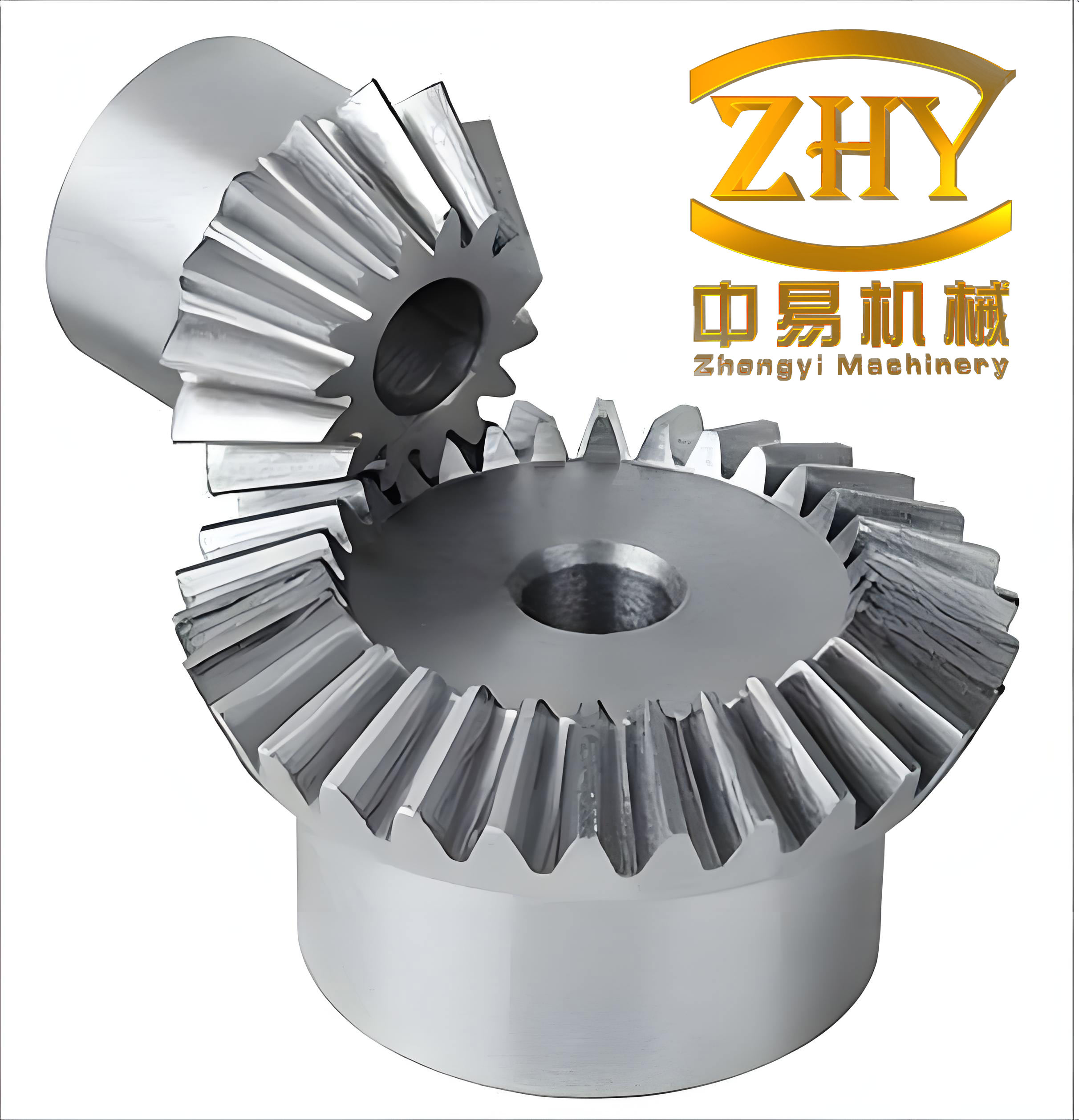
Straight bevel gears are essential components for transmitting motion and power between intersecting axes. Compared with spiral bevel gears, they possess simpler tooth profiles, which makes their design, manufacturing, and installation relatively easier. Consequently, they are widely applied in automotive, machine tool, and general machinery industries. However, the domestic manufacturing of straight bevel gears still predominantly employs traditional machines such as the Y236 planing machine and the Y2726 double-head milling machine. These mechanical machines are characterized by complex transmission chains, poor rigidity, difficult adjustment, and intermittent indexing processes. Such limitations significantly hinder the development and broader application of straight bevel gears.
In contrast, spiral bevel gear manufacturing has advanced significantly with the introduction of CNC Free-form machines. The Gleason Phoenix series and Oerlikon machines exemplify modern flexible manufacturing systems capable of producing various gear types with high precision and efficiency. Moreover, Gleason has successfully adapted its Free-form machines for straight bevel gears using Coniflex tools, claiming productivity improvements of 100% to 120% compared with conventional mechanical machines. The Italian company Samputensili has also achieved continuous machining of straight bevel gears using specially designed cutter heads.
Despite these international developments, detailed technical information remains proprietary. In China, limited research has been conducted on advanced machining methods specifically tailored for straight bevel gears. My research group at Tianjin University has long been devoted to the study of cycloidal rotational indexing (rotary indexing) machining technology. We have successfully applied this technology to machining synchronizer hub chamfers and sliding slots. Building upon our accumulated knowledge, I proposed the application of the rotational indexing principle to the continuous machining of straight bevel gears.
2 Fundamentals of Straight Bevel Gears
2.1 Gear Geometry and Basic Parameters
Straight bevel gears transmit motion between intersecting shafts. The relative motion of the two gears can be considered as pure rolling of two pitch cones with a common apex. For an orthogonal shaft arrangement with a 90° shaft angle, the pitch cone angles are determined by the gear ratio. The basic geometric parameters include the module m at the large end, the number of teeth z, the pressure angle α, the pitch cone angle δ, the face width B, and the cone distance R.
Table 1 lists the basic geometric parameters of a typical straight bevel gear used in my case study. These parameters were selected based on a practical engineering application to validate the proposed machining method.
| Symbol | Parameter | Value |
|---|---|---|
| z | Number of teeth | 25 |
| m | Large-end module (mm) | 3 |
| α | Pressure angle (°) | 20 |
| δ | Pitch cone angle (°) | 45 |
| B | Face width (mm) | 18 |
| R | Cone distance (mm) | 53 |
| ha | Addendum (mm) | 3 |
| hf | Dedendum (mm) | 3.6 |
| δa | Face cone angle (°) | 48°15′ |
| δf | Root cone angle (°) | 40°25′ |
In the design of straight bevel gears, the gear tooth profile is theoretically a spherical involute. The theoretical tooth flank of a straight bevel gear is formed by rolling a plane tangent to the base cone. The spherical involute is the intersection of the involute cone surface with a sphere centered at the cone apex. In practice, the spherical involute is often approximated by the octoid or the involute in the back cone, leading to inevitable manufacturing errors. For my research, I directly adopted the theoretical spherical involute as the evaluation reference to achieve the highest possible accuracy.
2.2 Theoretical Tooth Flank Equation
The involute cone surface of a straight bevel gear can be expressed in a fixed coordinate system O-xyz with the origin at the cone apex and the z-axis along the base cone axis. Using the coordinate transformation between the fixed frame and a moving frame O-x₁y₁z₁, the tooth flank equation of the straight bevel gear is derived as:
$$ \begin{cases} x = r(\cos\psi \sin\gamma \cos\phi + \sin\psi \sin\phi) \\ y = r(\cos\psi \sin\gamma \sin\phi – \sin\psi \cos\phi) \\ z = r\cos\psi \cos\gamma \end{cases} $$
Here, r is the radial parameter, φ is the angle between O’N and O’A, γ is the base cone angle satisfying sinγ = cosα sinδ, and ψ is the angle between the radius OK and the instantaneous rotation axis ON, with sinψ = sinφ sinγ.
When r equals the outer cone distance R, the trajectory of the spherical involute at the large end is obtained. This equation provided the theoretical basis for evaluating the tooth flank accuracy in my subsequent analysis of the rotational indexing machining process.
3 Rotational Indexing Machining Principle for Straight Bevel Gears
3.1 Concept of Rotational Indexing Machining
Rotational indexing machining, also called rotary indexing or continuous indexing machining, is a material removal process in which the workpiece rotates continuously and the cutter also rotates synchronously. Cutting and indexing are accomplished concurrently during the rotational motion. This method eliminates the separate indexing step typical of conventional single-index machining, thereby significantly improving productivity. When the cutting point trajectory follows a cycloidal or spatial curve, the technique is referred to as cycloidal rotational indexing machining.
In the machining of straight bevel gears, my key idea is to position the cutter head such that the cutting point trajectory approximates the straight generatrix of the conical surface. The relative motion between the cutter head and the workpiece yields a spatial curve. By carefully selecting and optimizing the machining parameters, a segment of this spatial curve can be made to closely match the straight line on the pitch cone or the root cone of the straight bevel gear.
3.2 Derivation from Epicycloid Bevel Gear Machining
The machining of epicycloid bevel gears is based on a virtual crown gear or generating gear. The cutter head rotates about its own axis while its center revolves around the axis of the generating gear. The relative motion of a cutting point on the cutter head with respect to the generating gear traces an extended epicycloid. In my proposed method for straight bevel gears, I do not rely on a virtual generating gear. Instead, the cutter head rotates about its own axis, the workpiece rotates about its axis, and the cutter head undergoes an additional tilting motion about a reference axis. This combination yields a spatial trajectory that can approximate a straight generatrix on the cone surface of a straight bevel gear.
Figure 1 illustrates the fundamental concept. A point M on the cutting edge starts cutting from the small end of the conical workpiece blank. Owing to the conical geometry, the point M would gradually move away from the cone surface as the cutter head rotates. To prevent this, I introduced a tilt angle β of the cutter head about a reference line l. By varying β from 0 to βmax during the cutting process, the cutting point can be maintained in close proximity to the cone surface, thus generating a trajectory that closely follows the generatrix of the cone.
3.3 Layout of Tool and Workpiece
The layout of the tool and workpiece is critical to the success of the proposed machining method. Initially, the cutter head axis and the workpiece axis are positioned at an angle of 90° + θ, where θ is defined as the workpiece swing angle. The cutting edge point M is located at a radius e (the cutter head radius) and is defined by the cutter position angle φ. The workpiece rotates at an angular velocity ω₂ which is synchronized with the cutter head angular velocity ω₁ through a fixed speed ratio η = ω₁/ω₂.
The machining motion consists of the following components:
- Cutter head rotation about its own axis, angular velocity ω₁
- Workpiece rotation about its own axis, angular velocity ω₂, with η = ω₁/ω₂
- Cutter head tilting (swinging) about the reference axis l, with the tilt angle β varying linearly
In this process, a cutter head with multiple groups of blades is used. Each group typically contains three blades: a roughing blade, an outside cutting blade, and an inside cutting blade. One blade machines the left tooth flank of a tooth gap, while another machines the right flank. The continuous rotation of the cutter head and workpiece enables the machining of successive tooth gaps without intermittent indexing. In this way, straight bevel gears can be machined with high efficiency.
4 Mathematical Model of Rotational Indexing Machining
4.1 Coordinate Systems and Transformations
To formulate the mathematical model of the cutting point trajectory, I established multiple coordinate systems. S₁ = {O₁; X₁, Y₁, Z₁} is the initial coordinate system of the cutter head, S₂ = {O₂; X₂, Y₂, Z₂} is the workpiece coordinate system, and S₃ = {O₃; X₃, Y₃, Z₃} represents the cutter head coordinate system after tilting by angle β about the reference line l.
The coordinate transformation from S₃ to S₂ is obtained by multiplying the individual transformation matrices:
$$ \begin{bmatrix} x_2 \\ y_2 \\ z_2 \\ 1 \end{bmatrix} = M_{21} \cdot M_{13} \cdot \begin{bmatrix} x_c \\ y_c \\ z_c \\ 1 \end{bmatrix} $$
where (x_c, y_c, z_c) are the coordinates of point M in the moving cutter head coordinate system, given by:
$$ x_c = e\sin\varphi, \quad y_c = e\cos\varphi, \quad z_c = 0 $$
The transformation matrix M₂₁ from S₁ to S₂ involves the workpiece rotation angle α₂ and the positional offsets, while M₁₃ from S₃ to S₁ involves the tilt angle β. The position of the cutter head center O₃ relative to the workpiece cone apex O₂ is expressed by coordinates (H, L, S) in the S₁ system:
$$ H = -R’ – B – e\sin\varphi, \quad L = -e\cos\varphi\cos\beta, \quad S = e\cos\varphi\sin\beta $$
where R’ = R – B (the inner cone distance). Substituting all transformation matrices and simplifying yields the parametric equation of the cutting point trajectory in the workpiece coordinate system, which I denote as the fundamental equation of the rotational indexing machining model for straight bevel gears:
$$ \begin{cases} x = f_1(\alpha_1, \eta, k_\alpha, e, \beta_{\max}, \varphi, \theta) \\ y = f_2(\alpha_1, \eta, k_\alpha, e, \beta_{\max}, \varphi, \theta) \\ z = f_3(\alpha_1, \eta, k_\alpha, e, \beta_{\max}, \varphi) \end{cases} $$
4.2 Parameter Analysis
The cutting point trajectory curve is governed by several independent parameters. The tool rotation angle α₁ is the parameter variable. The workpiece rotation angle is α₂ = η α₁. The cutter tilt angle β varies linearly with α₁ according to:
$$ \beta = \beta_{\max} \cdot \frac{\alpha_1}{\alpha_{\max}} $$
The maximum tool rotation angle αmax is related to the face width B and the cutter radius e by:
$$ \alpha_{\max} = k_\alpha \cdot \frac{B}{e} $$
where kα is the maximum tool rotation angle coefficient. The speed ratio η is determined by the gear tooth number z and the cutter group number z₁:
$$ \eta = \frac{z_1 k_z}{z} $$
where kz is the number of teeth crossed between successive cutter groups, a positive integer not divisible by z to ensure all teeth are machined.
The cutter radius e must satisfy both geometric and practical constraints:
$$ \frac{\pi z_1 B}{2} \leq e \leq 4B $$
Table 2 summarizes the parameters used in the mathematical model along with their definitions and ranges.
| Parameter | Symbol | Definition and range |
|---|---|---|
| Workpiece swing angle | θ | Between root angle δf and face angle δa |
| Speed ratio | η | η = z₁k_z/z |
| Tool radius | e | πz₁B/2 ≤ e ≤ 4B |
| Max tool angle | αmax | αmax = kα·B/e, kα ≥ 1 |
| Cutter position angle | φ | Determined by geometric relations |
| Max tilt angle | βmax | Typically between 5° and 10° |
4.3 Cutter Position Angle and Maximum Tilt Angle
The cutter position angle φ can be derived from the geometric relation that the trajectory chord length should approximate the face width. Considering the triangle formed by the trajectory endpoints and the origin, I derived:
$$ \varphi = \frac{\alpha_{\max}}{2} – \arccos\left( \frac{e^2 + B^2 – (2R\sin(\eta\alpha_{\max}/2)\sin\theta)^2}{2eB} \right) – \frac{\alpha_{\max}}{2} + \frac{\pi}{2} $$
The maximum tilt angle βmax is obtained from the condition that the trajectory endpoint lies on the cone surface. Equating the perpendicular distance from the endpoint to the tangent plane with the cone surface deviation, I obtained:
$$ \beta_{\max} = \arcsin\left( \frac{R \sin\theta \cos\theta \left[ 1 – \cos(\eta\alpha_{\max}) \right]}{2e \sin(\alpha_{\max}/2) \sin(\varphi + \alpha_{\max}/2)} \right) $$
These expressions demonstrate that the cutter position angle and maximum tilt angle are not independent but are functions of the other machining parameters. Therefore, the key design variables that remain to be optimized are the speed ratio η, the tool radius e, and the coefficient kα. After optimization, the derived parameters φ and βmax are calculated accordingly.
5 Parameter Optimization
5.1 Straightness Error Evaluation
To quantify how closely the cutting point trajectory approximates the straight generatrix of the cone surface, I introduced a straightness error metric μ. For the trajectory segment AB that is intended to approximate the generatrix, the straightness error is defined as the radius of the smallest cylinder centered on the ideal generatrix that completely encloses the trajectory segment.
In the workpiece coordinate system, the generatrix of the cone at radius R is a straight line segment described by:
$$ x = kz, \quad y = 0, \quad R – B \leq \sqrt{x^2 + z^2} \leq R $$
The distance from a point on the cutting trajectory to this line is computed using the point-to-line distance formula. Since the trajectory is defined parametrically, the distance d is a function of the tool rotation angle α₁ and the machining parameters:
$$ d = f(\alpha_1, \eta, k_\alpha, e) $$
The straightness error is the maximum value of d over the trajectory segment:
$$ \mu = \max(d) $$
This error can be compared with the tooth trace tolerance specified in the gear accuracy standard. Table 3 lists the allowable tooth trace tolerances for bevel gears of various accuracy grades and face widths. For my case study with face width B = 18 mm and accuracy grade 7, the allowable tolerance is 16 μm.
| Face width B (mm) | Accuracy grade 5 | Grade 6 | Grade 7 | Grade 8 | Grade 9 | Grade 10 |
|---|---|---|---|---|---|---|
| <5 | 4 | 5 | 6 | 8 | 10 | 12 |
| 5~10 | 6 | 8 | 10 | 12 | 16 | 20 |
| >10 | 10 | 12 | 16 | 20 | 25 | 32 |
5.2 Sensitivity Analysis
I analyzed the influence of each independent parameter on the straightness error μ. The results are summarized as follows:
Influence of speed ratio η: As η increases from a small value, the straightness error first decreases and then increases, exhibiting a clear minimum. The optimal η value depends on the other parameters.
Influence of tool radius e: The straightness error decreases rapidly with increasing e at small values and then stabilizes. Once e exceeds a threshold, the error is essentially constant and satisfies the accuracy requirement. In practice, the smallest e value that meets the accuracy is preferred to minimize machine size and cost.
Influence of coefficient kα: For kα in the range of 1 to about 1.15, the straightness error remains relatively small. Beyond this range, the error increases sharply. Therefore, kα should be limited to approximately 1 to 1.15 to maintain acceptable accuracy.
Figure 2 provides a comparison of the relative influence of η and e on the straightness error. When e is varied from 40 to 70 mm, the minimum μ changes from 0.0819 to 0.0686, with the smallest value 0.0069 occurring at e = 55 mm. When η is varied from 0.72 to 0.56, the minimum μ changes from 0.0069 to 0.2283. This comparison shows that the speed ratio η has a stronger influence on the straightness error than the tool radius e. The coefficient kα has the least influence among the three parameters.
5.3 Optimization Method
Based on the sensitivity analysis, I formulated the parameter optimization problem as a minimax optimization problem:
$$ \min_{\eta, e, k_\alpha} \left\{ \max_{\alpha_1 \in [0, \alpha_{\max}]} d(\alpha_1, \eta, k_\alpha, e) \right\} $$
Subject to the constraints:
$$ \begin{cases} 0 \leq \alpha_1 \leq \alpha_{\max} \\ \eta = z_1 k_z / z, \quad k_z = 1, 2, 3, 4 \\ \pi z_1 B / 2 \leq e \leq 4B \\ 1 \leq k_\alpha \leq (\pi/2 – \varphi) e / B \end{cases} $$
I utilized the fminimax function in MATLAB to solve this optimization problem. The optimization procedure iteratively adjusts the parameters η, e, and kα and computes the straightness error until the minimum is found or the error falls below the allowable tolerance. Figure 3 shows a comparison of the trajectory segment before and after optimization. The optimized curve segment AB₁ is significantly closer to the ideal generatrix than the initial segment AB.
6 Tooth Surface Generation and Cutting Edge Modification
6.1 Forming Method for Tooth Surface Generation
Once the cutting point trajectory is optimized to approximate the generatrix on the cone surface, the next step is to generate the tooth flank of the straight bevel gear. I adopted the forming method (also called the profiling method), in which the cutting edge is shaped as the small-end spherical involute of the theoretical tooth flank. The cutting edge moves along the optimized cutting point trajectory, sweeping out the entire tooth flank.
The workpiece is mounted such that its root cone angle θ equals the root angle δf. The spherical involute cutting edge is transformed from the workpiece coordinate system to the cutter head coordinate system using the inverse coordinate transformation derived in Section 4. The cutting edge equation in the cutter head coordinate system is obtained as:
$$ \begin{cases} x_c = (R-B)(\cos\psi \sin\gamma \cos\phi + \sin\psi \sin\phi)\sin\theta + z_c \cos\theta + e\sin\varphi – (R-B) \\ y_c = -(R-B)(\cos\psi \sin\gamma \sin\phi – \sin\psi \cos\phi) + e\cos\varphi \\ z_c = -(R-B)(\cos\psi \sin\gamma \cos\phi + \sin\psi \sin\phi)\cos\theta + (R-B)\cos\psi \cos\gamma \sin\theta \end{cases} $$
The tooth flank is then mathematically expressed by combining the cutting edge equation with the cutting point trajectory equation:
$$ \begin{cases} x = g_1(\alpha_1, \phi, \eta, e, k_\alpha) \\ y = g_2(\alpha_1, \phi, \eta, e, k_\alpha) \\ z = g_3(\alpha_1, \phi, \eta, e, k_\alpha) \end{cases} $$
This is a parametric surface in two parameters: the tool rotation angle α₁ and the spherical involute parameter φ.
6.2 Tooth Flank Error Evaluation
To evaluate the accuracy of the machined tooth flank, I computed the distance from points on the machined flank to the theoretical involute cone surface. The theoretical tooth flank equation is known from Section 2.2. For each point on the machined flank, the minimum distance to the theoretical flank is found by solving the coupled equations:
$$ \begin{cases} \frac{\partial d^2}{\partial r} = 0 \\ \frac{\partial d^2}{\partial \phi} = 0 \end{cases} $$
These equations reduce to a system of two nonlinear algebraic equations in r and φ. Solving this system and substituting back yields the minimum distance d. The tooth flank error Δ is defined as the maximum of these minimum distances over the entire machined flank:
$$ \Delta = \max(d) $$
For the initial cutting edge shaped as a spherical involute, I calculated the tooth flank error to be 0.0564 mm. This value exceeds the typical allowable error of 0.02 mm for the specified accuracy grade. Therefore, cutting edge modification is necessary to reduce the tooth flank error.
6.3 Cutting Edge Modification Using Backtracking Method
I developed a systematic procedure for modifying the cutting edge to minimize the tooth flank error. The procedure involves the following steps:
- Discretize the spherical involute cutting edge into a series of edge points.
- For each edge point, compute its trajectory curve when moving along the optimized cutting path.
- Calculate the maximum deviation of each trajectory from the theoretical tooth flank.
- If the maximum deviation for a point is below the allowable error, designate it as a retained point.
- Otherwise, designate it as a point to be modified.
- For each point to be modified, find the point on its trajectory with the maximum deviation. Take the midpoint between this point and its perpendicular foot on the theoretical flank. Back-calculate the corresponding new edge point.
- Repeat the process until all modified points have deviations below the allowable threshold.
- Fit the new set of edge points using the least-squares polynomial method to obtain the modified cutting edge equation.
In my case study, the spherical involute cutting edge was discretized into 13 points. Only the 4 points near the root of the tooth had deviations exceeding 0.02 mm and thus required modification. To improve fitting accuracy, these 4 edge segments were further refined into 8 points. Using the backtracking method, 8 new edge points were generated. Table 4 lists the coordinates of the cutting edge points before and after modification.
| Point | Original x_c | Original y_c | Original z_c | Modified x_c | Modified y_c | Modified z_c |
|---|---|---|---|---|---|---|
| 1 | 16.5883 | 51.3890 | -0.0007 | 16.5282 | 51.4775 | 0.0013 |
| 2 | 16.5882 | 51.3861 | -0.0668 | 16.5078 | 51.4002 | -0.0997 |
| 3 | 16.5879 | 51.3772 | -0.1695 | 16.4795 | 51.3592 | -0.2224 |
| 4 | 16.5873 | 51.3661 | -0.2640 | 16.4510 | 51.3170 | -0.3411 |
| 5 | 16.5862 | 51.3495 | -0.3789 | 16.4224 | 51.2720 | -0.4699 |
| 6 | 16.5854 | 51.3388 | -0.4440 | 16.3939 | 51.2301 | -0.5739 |
| 7 | 16.5845 | 51.3264 | -0.5141 | 16.3654 | 51.1873 | -0.6804 |
| 8 | 16.5832 | 51.3121 | -0.5891 | 16.3366 | 51.1435 | -0.7892 |
| 9 | 16.5725 | 51.2081 | -1.0370 | 16.5725 | 51.2081 | -1.0370 |
| 10 | 16.5499 | 51.0391 | -1.6005 | 16.5499 | 51.0391 | -1.6005 |
| 11 | 16.5095 | 50.7916 | -2.2705 | 16.5095 | 50.7916 | -2.2705 |
| 12 | 16.4438 | 50.4539 | -3.0366 | 16.4438 | 50.4539 | -3.0366 |
| 13 | 16.3447 | 50.0161 | -3.8868 | 16.3447 | 50.0161 | -3.8868 |
| 14 | 16.2034 | 49.4706 | -4.8077 | 16.2034 | 49.4706 | -4.8077 |
| 15 | 16.0105 | 48.8122 | -5.7854 | 16.0105 | 48.8122 | -5.7854 |
| 16 | 15.7565 | 48.0382 | -6.8050 | 15.7565 | 48.0382 | -6.8050 |
| 17 | 15.4317 | 47.1485 | -7.8513 | 15.4317 | 47.1485 | -7.8513 |
The 17 modified edge points were then fitted using the least-squares polynomial method. I performed a fourth-degree polynomial fit for both xc(zc) and yc(zc), resulting in the modified cutting edge equation:
$$ \begin{cases} x_c = 16.5158 – 0.0532z_c – 0.0246z_c^2 – 0.0006z_c^3 – 4.4\times10^{-4}z_c^4 \\ y_c = 51.4338 + 0.15z_c – 0.0642z_c^2 – 0.0028z_c^3 – 1.38\times10^{-4}z_c^4 \end{cases} $$
Table 5 summarizes the errors before and after each stage of the machining process.
| Stage | Straightness error μ / Tooth flank error Δ (mm) | Allowable (mm) | Status |
|---|---|---|---|
| Initial cutting point trajectory on pitch cone | μ = 0.0068 | 0.016 | Satisfactory |
| Tooth flank with spherical involute edge | Δ = 0.0564 | 0.02 | Needs modification |
| Tooth flank with modified cutting edge | Δ = 0.0188 | 0.02 | Satisfactory |
7 Case Study and Results
7.1 Workpiece Specifications
To validate the proposed rotational indexing machining method for straight bevel gears, I conducted a detailed computational case study on a gear with the following specifications:
- Number of teeth: z = 25
- Module at large end: m = 3 mm
- Pressure angle: α = 20°
- Pitch cone angle: δ = 45°
- Face width: B = 18 mm
- Cone distance: R = 53 mm
- Root cone angle: δf = 40°25′
- Face cone angle: δa = 48°15′
7.2 Optimization of the Cutting Point Trajectory
I first targeted the generatrix on the pitch cone as the object to be approximated. At this stage, the workpiece swing angle θ equals the pitch cone angle δ = 45°. Using the minimax optimization procedure described earlier, I obtained the optimal machining parameters listed in Table 6.
| Parameter | Symbol | Value |
|---|---|---|
| Max tool angle coefficient | kα | 1.1053 |
| Speed ratio | η | 0.72 |
| Tool radius (mm) | e | 54 |
| Cutter position angle (°) | φ | 19.39 |
| Max tilt angle (°) | βmax | 5.39 |
| Straightness error (mm) | μ | 0.0068 |
The optimized straightness error of 6.8 μm is well below the allowed tooth trace tolerance of 16 μm for grade 7 accuracy. This result confirms that the spatial curve trajectory can approximate the straight generatrix on the pitch cone within acceptable accuracy limits.
7.3 Tooth Flank Generation and Modification
With the optimized parameters, I proceeded to generate the tooth flank using the forming method. The workpiece was positioned at the root cone angle δf = 40°25′. The initial cutting edge was taken as the spherical involute. The generated tooth flank showed an error distribution characterized by larger deviations near the root and tip, with a maximum tooth flank error of 0.0564 mm.
After applying the backtracking modification method and least-squares polynomial fitting, the new cutting edge yielded a tooth flank error of Δ = 0.0188 mm. This value satisfies the 0.02 mm requirement, demonstrating the effectiveness of the cutting edge modification procedure. The new cutting edge scatters near the original spherical involute but manifests subtle corrections specifically in the root region, where the initial error was most pronounced.
7.4 Machine Settings and Machining Parameters
Table 7 presents the final machine settings and machining parameters required to implement the rotational indexing machining of straight bevel gears on a Free-form machine.
| Type | Parameter | Symbol | Value |
|---|---|---|---|
| Machine setting | Workpiece swing angle | θ | 40°25′ |
| Machine setting | Cutter position angle | φ | 17.48° |
| Machine setting | Horizontal offset O₂A | O₂A | 51.5 mm |
| Machine setting | Vertical offset O₂C | O₂C | 18.78 mm |
| Machining parameter | Speed ratio | η | 0.72 |
| Machining parameter | Tool radius | e | 54 mm |
| Machining parameter | Max tilt angle | βmax | 5.68° |
| Machining parameter | Cutter groups | z₁ | 9 |
| Machining parameter | Crossed teeth | kz | 2 |
8 Implementation on Free-form CNC Machines
Although the rotational indexing machining principle requires three rotational motions — namely, the workpiece rotation, the cutter head rotation, and the cutter head tilting about the reference axis — the tilting motion can be transformed into translational motions to enable implementation on standard Free-form six-axis CNC machines. Since the tilting axis l is parallel to the x-axis, the tilting motion can be decomposed into equivalent motions along the y-axis and z-axis.
During the cutting phase from time t = 0 to t₁ (where t₁ = αmax/ω₁), the y and z axis motions follow:
$$ \begin{cases} \Delta y = e[\cos\varphi – \cos(\varphi+\omega_1 t)]\cdot[1-\cos(\beta_t)] \\ \Delta z = e[\cos\varphi – \cos(\varphi+\omega_1 t)]\cdot\sin(\beta_t) \end{cases} $$
During the rapid return phase from t₁ to t₂ (where t₂ = 2π z₁/(zω₁)), the y and z axes return to their original positions with opposite velocities. Thus, by programming the coordinated motions of two rotational axes (workpiece axis A and cutter head axis C) and two translational axes (Y and Z), the rotational indexing machining of straight bevel gears can be realized directly on a Free-form machine. This motion transformation greatly expands the applicability of the proposed method without requiring the development of entirely new machine structures.
9 Conclusions
In this research, I proposed and systematically investigated a novel rotational indexing machining method for straight bevel gears based on the principle of cycloidal rotational indexing. The main findings and contributions of my work are summarized as follows:
(1) Spatial curve approximation of straight lines. I successfully explained the machining principle of straight bevel gears using the mathematical concept of spatial curves approximating straight generatrices. The cutting point trajectory, derived from the relative motion between the cutter head and the workpiece, can form a segment that closely approximates the straight generatrix on the cone surface of a straight bevel gear. This approach extends the planar cycloidal principle to spatial geometry.
(2) Tilt angle compensation. I introduced a cutter head tilt angle β that varies during machining to compensate for the geometric deviation caused by the conical surface. This tilting motion ensures that the cutting edge remains in close proximity to the cone surface throughout the cutting process, which is essential for maintaining the desired tooth flank geometry of straight bevel gears.
(3) Mathematical model and optimization. I established the mathematical model of the rotational indexing machining process, namely the parametric equation of the cutting point trajectory. Through sensitivity analysis, I identified the speed ratio η and the tool radius e as the most influential parameters and developed a minimax optimization procedure to minimize the straightness error. The optimized trajectory reduces the straightness error to well below standard tolerances.
(4) Tooth flank generation and cutting edge modification. I realized the tooth flank generation of straight bevel gears using the forming method, in which the cutting edge is shaped as the spherical involute. I developed a backtracking method for cutting edge modification that effectively reduces the tooth flank error from above 0.05 mm to below 0.02 mm, satisfying the requirements of grade 7 accuracy. The proposed method offers a systematic approach for cutting edge design in the machining of straight bevel gears.
(5) Machine settings and Free-form implementation. I determined the complete set of machine adjustment parameters and machining parameters required for the rotational indexing machining of straight bevel gears. Through a motion transformation, I showed that the tilting motion can be equivalently realized by translational motions along the y and z axes, enabling direct implementation on existing Free-form six-axis CNC machines.
The computational case study confirmed the feasibility of the method. The straightness error of the optimized cutting point trajectory on the pitch cone was 6.8 μm, and the final tooth flank error after cutting edge modification was 18.8 μm, both within the allowable tolerances. These results demonstrate the correctness and practical viability of the proposed rotational indexing machining technology for straight bevel gears.
Several aspects warrant further investigation in future work. First, the parameter optimization should be refined by directly using the cutter blade group number and crossed teeth number as design variables rather than the speed ratio. Second, the machining of the right tooth flank of straight bevel gears should be studied with similarly detailed cutting edge design and error evaluation. Finally, gear pair contact analysis should be performed to account for the actual meshing and transmission performance of the machined gear pairs, which may necessitate additional flank modifications for optimal load distribution and noise characteristics.
In summary, this fundamental study provides a solid theoretical foundation for the development of continuous indexing machining technology for straight bevel gears. The proposed rotational indexing machining method has the potential to significantly enhance production efficiency compared with conventional intermittent processes, improve manufacturing accuracy, and contribute to the advancement of gear manufacturing technology. Future efforts focused on machine tool design, experimental validation, and process optimization will be essential to fully realize the industrial application of this technology.