
I have focused my work on the thin-spoke gear that is widely used in helicopter transmission systems, because this type of gear combines low weight with high speed and high load capacity. In practical gear cutting, the thin spoke is a weak rigid structure. When I machine the spoke by turning, the spoke often deforms, the parallelism and circularity deviate excessively, and the hub region becomes eccentric. This eccentricity later causes unbalanced vibration in the transmission. My aim is therefore to understand the deformation mechanism in gear cutting, to predict the deformation with finite element simulation, and to propose a clamping strategy that reduces the final distortion.
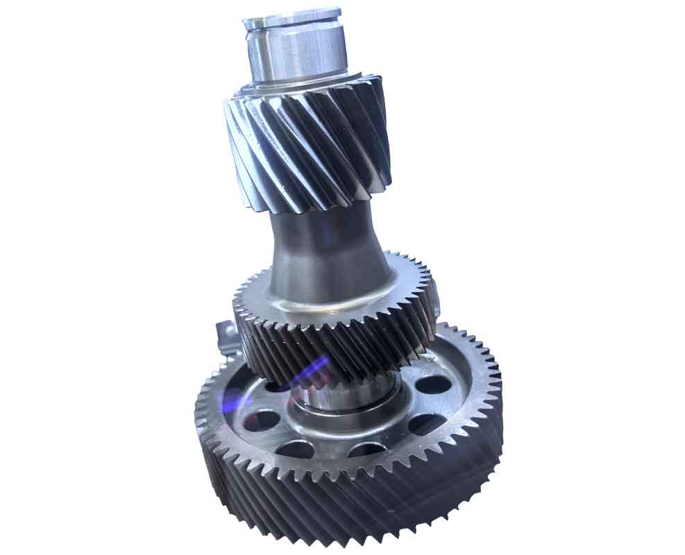
I treat the problem as a coupled thermal-mechanical gear cutting problem. The workpiece material is 18Cr2Ni4WA medium carbon steel, which is a high-strength carburizing steel. It has good toughness and hardenability, but it is also difficult to cut because the chip is long and the cutting force is high. In my study, the spoke is machined with an end-face grooving tool. The tool removes material in the axial direction, and the remaining spoke thickness is only a few millimeters. I use finite element simulation, cutting experiments, and clamping experiments together so that the predicted deformation can be compared with measured deformation.
Material Model and Geometry
I first established the material data required for gear cutting simulation. The chemical composition of 18Cr2Ni4WA steel is summarized in Table 1. The mechanical properties are listed in Table 2. These properties are used in the thermo-mechanical coupled model.
| Element | Ni | Cr | W | Mn | Si | C | P | S | Fe |
|---|---|---|---|---|---|---|---|---|---|
| Content (%) | 4.13 | 1.48 | 0.88 | 0.35 | 0.26 | 0.18 | 0.012 | 0.011 | Balance |
| Property | Density (kg/m3) | Young’s modulus (GPa) | Poisson’s ratio | Yield strength (MPa) | Thermal conductivity (W/m·K) | Thermal expansion (K-1) | Specific heat (J/kg·K) |
|---|---|---|---|---|---|---|---|
| Value | 7910 | 202 | 0.27 | 1800 | 44 | 1.24×10⁻⁵ | 460 |
For the dynamic behavior of the material in gear cutting, I adopted the Johnson-Cook constitutive model. The flow stress is expressed as:
$$\sigma = (A + B\varepsilon^n)\left(1 + C\ln\frac{\dot{\varepsilon}}{\dot{\varepsilon}_0}\right)\left[1 – \left(\frac{T-T_{room}}{T_{melt}-T_{room}}\right)^m\right]$$
In this equation, A is the yield strength, B is the strain hardening coefficient, C is the strain rate sensitivity, n is the hardening exponent, and m is the thermal softening exponent. The symbols T, Troom, and Tmelt denote the current temperature, room temperature, and melting temperature, respectively. The equivalent plastic strain is denoted by ε, and the equivalent plastic strain rate is denoted by ε̇. The reference strain rate is ε̇0.
I also used the Johnson-Cook damage model to simulate chip separation. The failure strain is written as:
$$\varepsilon_f = \left[D_1 + D_2\exp\left(D_3\frac{p}{\sigma}\right)\right]\left(1 + D_4\ln\frac{\dot{\varepsilon}}{\dot{\varepsilon}_0}\right)\left(1 + D_5\frac{T-T_{room}}{T_{melt}-T_{room}}\right)$$
The damage indicator is accumulated according to:
$$\omega = \sum \frac{\Delta\varepsilon}{\varepsilon_f}$$
When ω reaches unity, the element is considered damaged and is removed from the gear cutting model. The Johnson-Cook parameters and the damage parameters for 18Cr2Ni4WA steel are listed in Table 3.
| Parameter | A (MPa) | B (MPa) | C | n | m | D1 | D2 | D3 | D4 | D5 |
|---|---|---|---|---|---|---|---|---|---|---|
| Value | 1010 | 1409 | 0.04 | 0.67 | 1.2 | 0.09 | 0.46 | -1.95 | 0.002 | 0.44 |
The geometry of the thin-spoke gear is a rotational body. The outer diameter is 120 mm, the tooth width is 20 mm, and the hub diameter is 29 mm. The spoke machining region has a diameter of 100 mm. Before gear cutting of the spoke, the spoke thickness is 10 mm. After machining, the target thickness is 3 mm. If the thickness becomes less than 3 mm, severe chatter can occur. I therefore use a quarter model for the large deformation simulation to save computational cost, while the local gear cutting simulation uses two-dimensional and three-dimensional models to obtain cutting force and temperature.
Finite Element Modeling of Gear Cutting
I established both a two-dimensional and a three-dimensional finite element model for gear cutting. The two-dimensional model is used to study the cutting mechanism, chip formation, stress field, and temperature field. The three-dimensional model is used to obtain the full cutting force vector and realistic chip morphology. In both models, the tool is treated as a rigid body because the ceramic tool does not wear significantly in the short cutting time. The workpiece is treated as an isotropic material.
The contact between the tool and the chip is modeled with a Coulomb friction law. The friction stress is:
$$\tau_f = \mu p \quad \text{if} \quad \tau_f < \tau_{max}$$
$$\tau_f = \tau_{max} \quad \text{if} \quad \tau_f \ge \tau_{max}$$
The limiting shear stress is calculated from the von Mises equivalent stress as:
$$\tau_{max} = \frac{\sigma_s}{\sqrt{3}}$$
The friction coefficient μ is an important calibration parameter. I later calibrated it by comparing simulated cutting forces with measured cutting forces in gear cutting experiments.
For the two-dimensional model, the workpiece length is 1 mm, the chip layer thickness is 0.1 mm, the damage layer thickness is 0.01 mm, and the substrate thickness is 0.3 mm. I used a slanted quadrilateral mesh in the chip layer to reduce mesh distortion. The element type is CPE4RT. For the three-dimensional model, the mesh size in the circumferential direction is 0.0005 m, and the mesh size in the radial direction is 0.00025 m. The element type is C3D8RT. The analysis time for the two-dimensional model is 0.0003 s, and for the three-dimensional model it is 0.004 s. The bottom nodes of the workpiece are fixed, and the tool is constrained so that only the cutting velocity is applied.
Simulation Results for Gear Cutting
I analyzed the simulation results for the condition of cutting speed 180 m/min, feed 0.1 mm/r, and width 2 mm. The chip is formed after the damage layer reaches the failure criterion. The chip type is continuous. The equivalent stress is highest in the primary deformation zone, and it is lower in the secondary and tertiary deformation zones. The shear angle obtained from the simulation is approximately 37 degrees.
The temperature field shows that the highest temperature is not exactly at the tool tip. It is located on the rake face. The temperature on the rake face decreases more slowly than the temperature on the flank face. The maximum temperature in the cutting zone is around 480 °C for the selected condition. In gear cutting, this temperature affects the thermal softening of the workpiece and therefore changes the cutting force.
I also simulated the residual stress field on the machined surface. The simulation procedure includes four stages: cutting, unloading, constraint conversion, and cooling. In the cutting stage, the tool moves through the workpiece. In the unloading stage, the tool is retracted. In the constraint conversion stage, the fixed boundary condition is replaced by a few constraints that only prevent rigid body motion. In the cooling stage, the workpiece is cooled to room temperature. The residual stress in the cutting direction is compressive near the surface and becomes compressive at greater depth, while the residual stress in the tool width direction is mainly tensile. The distribution is spoon-shaped. The measured residual stresses are listed in Table 4, and the simulation error is within 10%.
| Residual stress component | Measured point 1 (MPa) | Measured point 2 (MPa) | Measured point 3 (MPa) | Measured point 4 (MPa) |
|---|---|---|---|---|
| X-direction stress | 612 | 670 | 563 | 558 |
| Z-direction stress | 1357 | 1443 | 1269 | 1223 |
The chip morphology in the three-dimensional simulation is smooth and spiral-shaped, which agrees with the actual chip obtained in gear cutting. The cutting force curves fluctuate after the steady state is reached. This fluctuation is caused by the competition between thermal softening and strain hardening. The average cutting force from the two-dimensional model is 539.5 N, while the average cutting force from the three-dimensional model is 553.6 N. The difference is 2.6%. The feed force from the three-dimensional model is 318.7 N, and the depth force is 44.13 N. Because the two-dimensional model cannot output the feed force, the three-dimensional model is preferred when the complete force vector is required.
| Model | Main cutting force (N) | Feed force (N) | Depth force (N) | Error in main force |
|---|---|---|---|---|
| 2D simulation | 539.5 | Not available | 36.1 | Reference |
| 3D simulation | 553.6 | 318.7 | 44.13 | 2.6% |
Cutting Force Measurement and Calibration
I carried out gear cutting experiments to measure the cutting force. The machine tool is a CNC lathe. The force measurement system consists of a piezoelectric dynamometer, a charge amplifier, a data acquisition card, and data processing software. The dynamometer is mounted between two base plates to measure three force components. The X-axis corresponds to the feed force, the Y-axis corresponds to the depth force, and the Z-axis corresponds to the main cutting force. The workpiece is a round bar with a diameter of 110 mm and a thickness of 30 mm. No cutting fluid is used. The experimental parameters are shown in Table 5.
| Level | Cutting speed vc (m/min) | Feed f (mm/r) | Width w (mm) |
|---|---|---|---|
| 1 | 90 | 0.06 | 1.8 |
| 2 | 120 | 0.08 | 2.0 |
| 3 | 180 | 0.10 | 2.2 |
| 4 | 270 | 0.12 | 2.4 |
| 5 | 360 | 0.14 | 2.6 |
From the single-factor experiments, I found that the main cutting force decreases slightly when the cutting speed increases. The feed force changes very little with cutting speed. At very high speed, the machine tool vibration causes abnormal force data. For the tested range, a cutting speed between 120 and 180 m/min is suitable for gear cutting of this material. The width and the feed have a stronger influence. The main cutting force increases almost linearly with the width. The feed force increases with the feed, but the increase is not exactly linear. When the feed is doubled, the main cutting force increases by about 45% to 55%. The depth force is mainly controlled by the side cutting edge and changes little with the width.
I calibrated the friction coefficient in the simulation with the measured cutting forces. Table 6 shows the design of the friction calibration. A friction coefficient of 0.2 gives the best agreement with the experiment and also matches the low friction characteristic of a ceramic tool.
| Case | Model | vc (m/min) | f (mm/r) | w (mm) | Friction coefficient μ |
|---|---|---|---|---|---|
| 1 | 3D | 180 | 0.10 | 2.0 | 0.2 |
| 2 | 3D | 180 | 0.10 | 2.0 | 0.3 |
| 3 | 3D | 180 | 0.10 | 2.0 | 0.4 |
| 4 | 3D | 180 | 0.10 | 2.0 | 0.5 |
| 5 | 3D | 180 | 0.10 | 2.0 | 0.6 |
| 6 | 3D | 180 | 0.10 | 2.0 | 0.8 |
The comparison between simulated and measured cutting forces is given in Table 7. The error is mostly within 15%, which confirms that the calibrated gear cutting model is reliable. The table also lists the simulated tool tip temperature. The maximum error appears in the depth force, because the side cutting edge contribution is difficult to capture exactly in the two-dimensional model.
| Test | vc level | f level | w level | Measured main force (N) | Simulated main force (N) | Error (%) | Measured feed force (N) | Simulated feed force (N) | Error (%) | Tool tip temperature (°C) |
|---|---|---|---|---|---|---|---|---|---|---|
| 1 | 1 | 3 | 2 | 548.6 | 566.3 | 3.22 | 348.5 | 333.8 | -4.22 | 412.5 |
| 2 | 2 | 3 | 2 | 539.9 | 560.7 | 3.85 | 344.3 | 327.4 | -4.91 | 442.5 |
| 3 | 3 | 3 | 2 | 526.2 | 553.6 | 5.21 | 340.3 | 318.7 | -6.35 | 479.9 |
| 4 | 4 | 3 | 2 | 506.6 | 531.9 | 4.99 | 337.9 | 310.4 | -8.14 | 519.6 |
| 5 | 5 | 3 | 2 | 501.9 | 529.3 | 5.46 | 374.3 | 307.2 | -17.92 | 548.5 |
| 6 | 3 | 1 | 2 | 382.9 | 389.1 | 1.62 | 300.2 | 291.3 | -2.96 | 455.3 |
| 7 | 3 | 2 | 2 | 449.0 | 465.7 | 3.72 | 322.4 | 303.8 | -5.77 | 461.8 |
| 8 | 3 | 3 | 2 | 526.2 | 553.9 | 5.21 | 340.3 | 318.7 | -6.35 | 510.9 |
| 9 | 3 | 4 | 2 | 569.7 | 586.5 | 2.95 | 347.5 | 326.3 | -6.10 | 479.9 |
| 10 | 3 | 5 | 2 | 624.3 | 643.9 | 3.14 | 356.4 | 339.7 | -4.69 | 477.5 |
| 11 | 3 | 3 | 1 | 472.2 | 491.7 | 4.12 | 312.4 | 295.1 | -5.54 | 464.2 |
| 12 | 3 | 3 | 2 | 526.2 | 553.6 | 5.21 | 340.3 | 318.7 | -6.35 | 479.9 |
| 13 | 3 | 3 | 3 | 555.8 | 586.9 | 5.59 | 376.6 | 350.5 | -6.93 | 491.2 |
| 14 | 3 | 3 | 4 | 595.9 | 654.7 | 9.87 | 393.7 | 364.6 | -7.39 | 498.5 |
| 15 | 3 | 3 | 5 | 663.3 | 710.9 | 7.18 | 448.6 | 415.6 | -7.36 | 512.3 |
Empirical Model for Gear Cutting Force
After the simulation model was calibrated, I used it to perform an orthogonal experiment. The empirical model for gear cutting force is assumed to have the following form:
$$F_c = C_{F_c} v_c^{a_1} f^{a_2} w^{a_3}$$
$$F_f = C_{F_f} v_c^{b_1} f^{b_2} w^{b_3}$$
Taking the logarithm of both sides gives:
$$\lg F = \lg C + a_1 \lg v_c + a_2 \lg f + a_3 \lg w$$
I designed a three-factor four-level orthogonal array. The factors and levels are shown in Table 8. Sixteen simulation cases were run, and the main cutting force and feed force were extracted. The results are listed in Table 9.
| Level | vc (m/min) | f (mm/r) | w (mm) |
|---|---|---|---|
| 1 | 90 | 0.06 | 1.8 |
| 2 | 110 | 0.08 | 2.0 |
| 3 | 130 | 0.10 | 2.2 |
| 4 | 150 | 0.12 | 2.4 |
| Run | vc (m/min) | f (mm/r) | w (mm) | Fc (N) | Ff (N) |
|---|---|---|---|---|---|
| 1 | 90 | 0.06 | 1.8 | 351.29 | 283.94 |
| 2 | 90 | 0.08 | 2.0 | 471.39 | 356.58 |
| 3 | 90 | 0.10 | 2.2 | 578.32 | 391.46 |
| 4 | 90 | 0.12 | 2.4 | 661.84 | 428.38 |
| 5 | 110 | 0.06 | 2.0 | 390.06 | 348.56 |
| 6 | 110 | 0.08 | 1.8 | 402.92 | 398.23 |
| 7 | 110 | 0.10 | 2.4 | 603.81 | 460.19 |
| 8 | 110 | 0.12 | 2.2 | 616.08 | 465.99 |
| 9 | 130 | 0.06 | 2.2 | 409.66 | 221.33 |
| 10 | 130 | 0.08 | 2.4 | 515.51 | 297.93 |
| 11 | 130 | 0.10 | 1.8 | 469.12 | 288.63 |
| 12 | 130 | 0.12 | 2.0 | 576.49 | 321.33 |
| 13 | 150 | 0.06 | 2.4 | 439.99 | 298.54 |
| 14 | 150 | 0.08 | 2.2 | 466.80 | 344.14 |
| 15 | 150 | 0.10 | 2.0 | 518.64 | 361.74 |
| 16 | 150 | 0.12 | 1.8 | 508.78 | 373.14 |
Using multiple linear regression, I obtained the following empirical equations for gear cutting force:
$$F_c = 1557.4 v_c^{-0.0729} f^{0.5814} w^{0.8320}$$
$$F_f = 4059.8 v_c^{-0.3228} f^{0.46} w^{0.2733}$$
The comparison between the predicted forces and the simulated forces is good. The empirical model shows that the width has the strongest effect on the main cutting force, followed by the feed, while the cutting speed has the weakest effect. This trend is useful for selecting parameters in gear cutting. When the same material removal rate is required, increasing the feed and reducing the width can lower the cutting force and reduce the risk of spoke deformation.
Deformation Prediction for the Thin Spoke
The thin spoke has low rigidity, so the cutting force and the clamping force both cause deformation. To predict the deformation, I used the element birth-death technique in ABAQUS. In this technique, the stiffness, mass, and load of a removed element are set to zero, which is equivalent to material removal. The analysis step is a coupled temperature-displacement step. The time for one element removal is calculated from the mesh size and the cutting speed:
$$T = \frac{10^{-3}L}{2\pi r V}$$
Here L is the element size in the circumferential direction, r is the radius of the machining position, and V is the rotational speed. The number of analysis steps is equal to the number of removed elements. Because the number of elements is large, I wrote a Python script to generate the analysis steps, add the model change keyword, and apply the moving load automatically.
The cutting force is applied as a surface traction. The equivalent nodal load is calculated by:
$$\{F\}^e = \int_S [N]^T \{q\} dS$$
Because the workpiece is rotational, the cutting force must be transformed into the global coordinate system. The transformation is:
$$\begin{bmatrix} F_x \\ F_y \\ F_z \end{bmatrix} = \begin{bmatrix} \cos\theta & -\sin\theta & 0 \\ \sin\theta & \cos\theta & 0 \\ 0 & 0 & 1 \end{bmatrix} \begin{bmatrix} F_z \\ F_y \\ F_x \end{bmatrix}$$
The angle θ changes from 0 to π/2 in the quarter model. The cutting heat is applied as a point heat source near the tool tip. I used the point-plane envelope method to determine the tool position and the corresponding element number. The flow of this method is as follows: I extracted the node coordinates and element connectivity from the input file, calculated the element center, and then checked whether the center was inside the element by using the six faces of the hexahedral element. For a face defined by four nodes, the plane equation is:
$$Ax + By + Cz + D = 0$$
For the element center p and a reference node outside the face, I calculated:
$$M_1 = Ax_0 + By_0 + Cz_0 + D$$
$$M_2 = Ax_8 + By_8 + Cz_8 + D$$
The product is:
$$F = M_1 M_2$$
If F is greater than zero, the center and the reference node are on the same side of the face. If F is less than or equal to zero, they are on opposite sides or on the face. By repeating this check for all faces, I identified the element that contains the tool position. This method allowed me to generate the tool path and the element removal sequence automatically.
I used a quarter model of the gear. The symmetry boundary conditions are applied on the two cut faces. The outer rim side and the hub inner wall are fully constrained to simulate the three-jaw chuck. After machining, the clamping constraints are removed, and only a few nodes are constrained to prevent rigid body motion. The initial temperature is room temperature. Because the material has high thermal conductivity, I treated the gear cutting process as adiabatic in the deformation model. The finite element flow includes geometry creation, mesh generation, node and element extraction, tool path calculation, load application, element removal, boundary condition setting, solution, and deformation extraction.
The cutting force and temperature load for different widths are listed in Table 10. The cutting speed is 180 m/min and the feed is 0.1 mm/r. The width varies from 1.8 mm to 2.6 mm.
| Case | vc (m/min) | f (mm/r) | w (mm) | Main force (N) | Feed force (N) | Depth force (N) | Tool tip temperature (°C) |
|---|---|---|---|---|---|---|---|
| 1 | 180 | 0.10 | 1.8 | 472 | 312 | 44 | 464 |
| 2 | 180 | 0.10 | 2.0 | 526 | 340 | 46 | 479 |
| 3 | 180 | 0.10 | 2.2 | 555 | 376 | 44 | 491 |
| 4 | 180 | 0.10 | 2.4 | 595 | 393 | 44 | 498 |
| 5 | 180 | 0.10 | 2.6 | 663 | 448 | 47 | 512 |
The stress field during gear cutting is concentrated near the hub. The maximum stress appears at the connection between the hub and the spoke, and it can exceed 1000 MPa. The minimum stress in the middle section of the spoke is about 163 MPa. After the tool path is completed, the temperature of the machined surface is higher than the temperature at the beginning of the cut. The heat conducts into the workpiece, but because the thermal conductivity is high, the surface temperature decreases quickly after the cut.
After the clamping constraints are released, the stress field is redistributed. The stress amplitude decreases, and part of the released stress appears as deformation. The maximum deformation occurs in the axial direction of the gear. The measured and simulated radial deformations are compared in Table 11. The simulation deformation is slightly larger than the measured deformation because the quarter model with symmetry constraints is stiffer than the real gear in some directions and softer in others. However, the trend is the same. The maximum simulated deformation is 0.0372 mm, and the maximum measured deformation is 0.0312 mm. The maximum prediction error is about 16%.
| Case | w (mm) | Simulated deformation (×10-2 mm) | Measured deformation (×10-2 mm) | Error (%) |
|---|---|---|---|---|
| 1 | 1.8 | 3.69 | 2.94 | 20.3 |
| 2 | 2.0 | 3.73 | 3.12 | 16.3 |
| 3 | 2.2 | 3.96 | 3.52 | 11.1 |
| 4 | 2.4 | 4.45 | 4.27 | -4.9 |
| 5 | 2.6 | 5.34 | 5.02 | 5.9 |
The circumferential parallelism deviation is also important. I measured the spoke at diameters of 33 mm, 53 mm, and 73 mm. The deformation is larger near the hub. This is because the outer part of the spoke is machined first, while the inner part still has more material and therefore higher rigidity. When the tool reaches the hub region, the spoke has already reached its final thickness, so it is more flexible. The measured parallelism deviation can be kept within about 30% of the simulated value. The deformation pattern is arc-shaped in the circumferential direction, with the maximum at the middle of the spoke. The quarter model cannot capture the full circumferential shape, but it still predicts the correct deformation trend.
The maximum deformation values for different widths are listed in Table 12. As the cutting force increases, the deformation increases. However, the deformation from 1.8 mm to 2.0 mm does not increase as much as expected. The reason is that a smaller width requires more passes to remove the same material, and each pass introduces residual stress near the hub. Therefore, a very small width is not always better. When the width is 2.6 mm, the main cutting force is 663 N, the feed force is 448 N, and the measured deformation is 0.0502 mm, which exceeds the tolerance of ±0.05 mm. To ensure the accuracy of the spoke in gear cutting, the main cutting force on the spoke surface should not exceed about 600 N.
| w (mm) | Main force (N) | Feed force (N) | Measured maximum deformation (×10-2 mm) |
|---|---|---|---|
| 1.8 | 472 | 312 | 2.94 |
| 2.0 | 526 | 340 | 3.12 |
| 2.2 | 555 | 376 | 3.52 |
| 2.4 | 595 | 393 | 4.27 |
| 2.6 | 663 | 448 | 5.02 |
Clamping Schemes and Their Effect on Deformation
I compared three clamping schemes for gear cutting of the thin-spoke gear. The first scheme is a three-jaw chuck. The second scheme is a special fixture that clamps the front and rear faces of the gear with double-end studs and bolts. The third scheme is a special fixture with an additional spoke support made of nylon. The support can be changed for different spoke thicknesses and diameters. The goal is to reduce the clamping deformation and the repeated positioning error.
I calculated the required clamping force from the cutting force. The formula is:
$$W_k = \frac{K F}{\mu}$$
Here K is the safety factor, F is the cutting force, and μ is the friction coefficient. For rough machining, K is between 2.5 and 3. For finish machining, K is between 1.5 and 2. I used K = 1.5. The machined outer surface has a friction coefficient of about 0.16. The maximum feed force is 448 N. The required clamping force is about 4200 N, which means about 1400 N on each jaw for the three-jaw chuck. For the special fixture, the feed force is balanced by the fixture, so only the main cutting force can cause circumferential slipping. The double-end stud has a nominal diameter of 12 mm, and its allowable clamping force is 5790 N. The corresponding maximum main cutting force is about 617.6 N. If the main cutting force exceeds this value, a keyway should be used to prevent slipping.
I simulated the clamping deformation of the three schemes. The three-jaw chuck applies a radial clamping force of 1400 N. The special fixture applies an axial clamping force of 5790 N. The simulation shows that the three-jaw chuck causes a larger spoke deformation because the radial force bends the thin spoke. The special fixture causes a smaller deformation because the clamping force is mainly axial. The fixture with a spoke support causes the smallest deformation because the support balances part of the cutting force and increases the local stiffness.
I then carried out gear cutting experiments with the three clamping schemes. The cutting parameters are vc = 180 m/min, f = 0.1 mm/r, and w = 2 mm. After machining, I measured the parallelism and flatness of the spoke with a coordinate measuring machine. For the parallelism measurement, I used 12 paths around the spoke. The datum plane was the rim surface at the same position as the measured surface. I determined the center of the gear from three fixed columns. Then I scanned each path with about 300 points. The parallelism results are shown in Table 13. The three-jaw chuck gives the largest parallelism error, and the special fixture gives the smallest. The fixture with spoke support gives a result between the two, but its deformation is the smallest because it balances the feed force.
| Clamping scheme | Parallelism error (mm) | Flatness error (mm) | Main observation |
|---|---|---|---|
| Three-jaw chuck | Largest | 0.0051 | Radial clamping bends the thin spoke |
| Special fixture | Smallest | 0.0026 | Axial clamping avoids radial bending |
| Special fixture with spoke support | Intermediate | 0.0049 | Support balances feed force but introduces slight axial load |
The flatness measurement was performed on a circular path at a diameter of 60 mm. The flatness error of the three-jaw chuck is 0.0051 mm. The flatness error of the special fixture is 0.0026 mm. The flatness error of the fixture with spoke support is 0.0049 mm. The special fixture gives the best flatness. The reason is that the machined residual stress is mainly tensile, and the thin spoke tends to bulge outward. The feed force is opposite to this bulging direction, so it can partially cancel the deformation. However, the radial clamping force of the three-jaw chuck adds an extra bending load, which doubles the flatness error compared with the special fixture.
From the experiments, I conclude that the special fixture is the best choice for gear cutting of the thin-spoke gear when the spoke thickness is not less than 3 mm. It reduces the clamping deformation, the repeated positioning error, and the final parallelism and flatness errors. If the cutting force is high, the fixture with spoke support can further reduce the absolute deformation, but the parallelism may be slightly worse. In that case, tool compensation based on the predicted deformation can be used together with the special fixture.
Discussion and Practical Recommendations
My study shows that gear cutting of a thin-spoke gear is controlled by several coupled factors: the cutting force, the cutting temperature, the residual stress, and the clamping force. The finite element model of gear cutting can predict the chip morphology, the cutting force, the temperature field, and the residual stress. The calibrated friction coefficient is 0.2. The empirical force model is reliable for the tested material and tool geometry. The deformation prediction model based on the element birth-death technique can capture the deformation trend of the thin spoke, although the quarter model gives a slightly conservative result.
For practical gear cutting, I recommend the following:
1. Use a cutting speed between 120 and 180 m/min for the end-face grooving operation. Higher speeds do not reduce the force significantly and can cause machine tool vibration.
2. Keep the main cutting force below about 600 N to avoid excessive spoke deformation. In the tested condition, this corresponds to a width of about 2.4 mm or less.
3. When the material removal rate must be maintained, increase the feed and reduce the width rather than increasing the width. The width has the strongest effect on the main cutting force.
4. Use a special fixture with axial clamping instead of a three-jaw chuck with radial clamping. The radial clamping force is a major cause of spoke bending.
5. If the spoke is very thin or the cutting force is high, add a nylon spoke support to the fixture. The support increases the local stiffness and balances part of the feed force.
6. For high-precision gear cutting, apply tool compensation based on the predicted deformation. The deformation is larger near the hub, so the compensation should be position-dependent.
Conclusion
I have developed a complete simulation and experimental framework for gear cutting of thin-spoke gears made of 18Cr2Ni4WA steel. The main conclusions are as follows.
First, the two-dimensional and three-dimensional gear cutting models can reproduce the chip formation, the temperature field, and the residual stress field. The two-dimensional model is efficient for studying the cutting mechanism, while the three-dimensional model is necessary for obtaining the complete cutting force vector. The difference in the main cutting force between the two models is only 2.6% for the tested condition.
Second, the friction coefficient between the ceramic tool and the workpiece was calibrated to 0.2. The simulated cutting forces agree with the measured forces within 15% for most conditions. The empirical equations for the main cutting force and the feed force were obtained by orthogonal simulation and multiple linear regression. The width has the strongest influence, followed by the feed, and the cutting speed has the weakest influence.
Third, the element birth-death technique and the point-plane envelope method were used to build a deformation prediction model for the thin spoke. The predicted deformation follows the same trend as the measured deformation. The maximum deformation occurs near the hub, and the circumferential deformation is arc-shaped. The main cutting force should be limited to about 600 N to keep the deformation within the tolerance.
Fourth, the clamping scheme strongly affects the final deformation. The three-jaw chuck causes the largest parallelism and flatness errors because of radial clamping. The special fixture with axial clamping gives the smallest errors. The fixture with a spoke support gives the smallest absolute deformation but a slightly larger parallelism error. For gear cutting of thin-spoke gears with a spoke thickness not less than 3 mm, the special fixture is the best compromise between accuracy and rigidity.
Overall, my work provides a practical method for predicting and controlling deformation in gear cutting of thin-spoke gears. The method combines material constitutive modeling, thermo-mechanical cutting simulation, force calibration, empirical force prediction, element removal simulation, and clamping optimization. It can be used to select cutting parameters, design fixtures, and compensate for deformation in the production of thin-spoke gears for helicopter transmissions.