
I focus on the chatter problem that appears during spiral bevel gear face hobbing. In this manufacturing process, the cutter head and the workpiece move in a coupled spatial relationship, and even a small relative vibration can alter the undeformed chip geometry, the instantaneous cutting force, and the final tooth surface. I therefore build a vectorized dynamic model for face hobbing, validate it with modal tests and industrial measurements, extract chatter-sensitive features by wavelet packet analysis, and finally identify stable cutting, transition, and chatter states by a one-versus-one multiclass support vector machine. The whole study is centered on gear hobbing because gear hobbing is the key operation that determines the surface quality, transmission noise, and service life of spiral bevel gears.
1. Engineering Background and Chatter Mechanism in Gear Hobbing
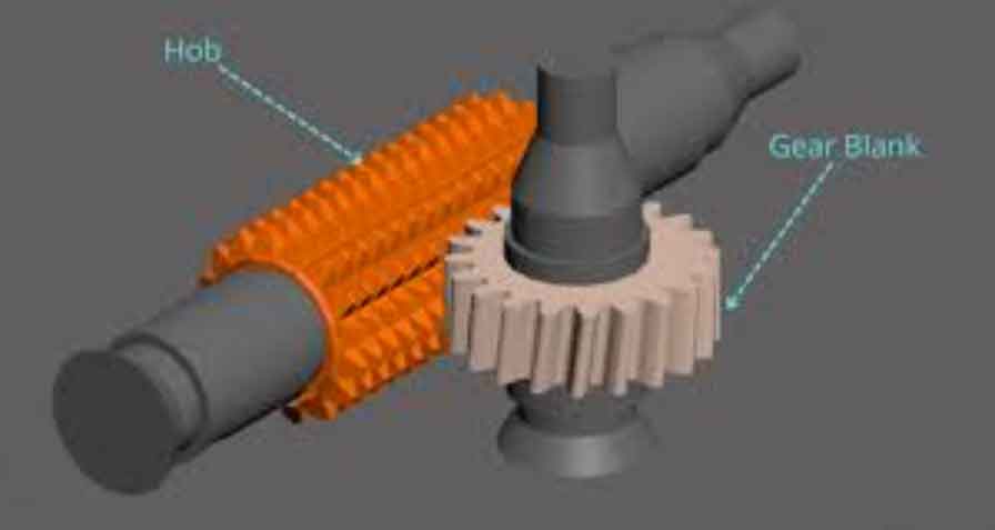
Spiral bevel gears are widely used in vehicle axles, helicopter transmissions, mining machinery, wind power systems, and high-speed rail equipment. Their tooth surfaces are complex, and their machining quality is strongly affected by the dynamic behavior of the gear hobbing process. In face hobbing, the cutter head rotates continuously while the workpiece rotates in a timed relationship. The cutting edges remove material from the gear blank along a generating motion. If the process loses stability, regenerative chatter appears, and the relative vibration between the tool and the workpiece becomes self-excited. This chatter leaves periodic ripples on the tooth surface, increases acoustic noise, accelerates tool wear, and can make the gear unacceptable.
I classify the chatter in gear hobbing into three main types: frictional chatter, mode-coupling chatter, and regenerative chatter. Frictional chatter can often be reduced by improving lubrication. Mode-coupling chatter can be reduced by structural redesign. Regenerative chatter, however, is generated by the interaction between the cutting process and the machine structure, and it is especially difficult to suppress in gear hobbing because the uncut chip thickness depends on the previous tooth surface. This regenerative effect is the core of my dynamic model.
The detection of chatter in gear hobbing usually follows four stages: data acquisition, signal processing, feature extraction, and state recognition. I follow the same logic but adapt each stage to spiral bevel gear face hobbing. Acceleration signals are collected from the cutter head in three orthogonal directions. Wavelet thresholding is used to remove noise. Time-domain, frequency-domain, and time-frequency features are compared. A wavelet packet energy entropy is proposed as a compact feature, and a support vector machine is trained to classify the cutting state. The target is not only to detect chatter after it occurs but also to distinguish a transition state before severe chatter fully develops.
2. Kinematic Relations of Gear Hobbing
I first describe the machine motion of spiral bevel gear face hobbing. The cutter head and the workpiece are connected through a series of coordinate transformations. The workpiece coordinate system is fixed to the gear blank, and the cutter head coordinate system is fixed to the rotating tool. Vibration displacements are introduced along the machine axes. The homogeneous transformation from the workpiece system to the cutter head system can be written as
$$
\mathbf{M}_{wh}=
\begin{bmatrix}
\cos\varphi_w & -\sin\varphi_w & 0 & X+x_w\\
\sin\varphi_w & \cos\varphi_w & 0 & Y+y_w\\
0 & 0 & 1 & Z+z_w\\
0 & 0 & 0 & 1
\end{bmatrix}
\begin{bmatrix}
\cos\beta_w & 0 & \sin\beta_w & 0\\
0 & 1 & 0 & 0\\
-\sin\beta_w & 0 & \cos\beta_w & 0\\
0 & 0 & 0 & 1
\end{bmatrix}
$$
Here, \(x_w\), \(y_w\), and \(z_w\) are the workpiece vibration components along the machine axes, while \(x_h\), \(y_h\), and \(z_h\) are the cutter head vibration components. The angles \(\varphi_w\) and \(\varphi_h\) represent the rotations of the workpiece and cutter head. The symbols \(X\), \(Y\), and \(Z\) denote the nominal machine settings of the cutter head. In gear hobbing, these settings control the generating motion and the contact condition between the cutting edges and the gear blank.
For the cutter head itself, the transformation from the cutter head coordinate system to the tool coordinate system is
$$
\mathbf{M}_{hT}=
\begin{bmatrix}
\cos\delta_T & -\sin\delta_T & 0 & R_1\\
\sin\delta_T & \cos\delta_T & 0 & h\\
0 & 0 & 1 & R_2\\
0 & 0 & 0 & 1
\end{bmatrix}
\begin{bmatrix}
1 & 0 & 0 & 0\\
0 & \cos\lambda & -\sin\lambda & 0\\
0 & \sin\lambda & \cos\lambda & 0\\
0 & 0 & 0 & 1
\end{bmatrix}
$$
where \(\delta_T\) is the mounting angle of the cutting tool, \(h\) is the reference height, \(R_1\) is the radial offset, \(R_2\) is the tangential radius, and \(\lambda\) is the inclined slot angle. The cutting edge geometry in the tool coordinate system is expressed as
$$
\mathbf{r}_T(s)=\left[\sin\alpha_b,\ \sin\alpha \tan\alpha_b,\ \cos\alpha,\ 1\right]^T s
$$
where \(\alpha_b\) is the profile angle of the cutting edge, \(\alpha\) is the rake angle, and \(s\) is the arc-length parameter. Combining the transformations gives the tooth surface of the spiral bevel gear generated by the forming method under the influence of cutting vibration:
$$
\mathbf{r}^{(W)}(s,\varphi)=\mathbf{M}_{wh}\mathbf{M}_{hT}\mathbf{r}_T(s)
$$
This vectorized expression is important for gear hobbing because it allows the instantaneous tooth surface to be updated with the vibration state. Instead of treating vibration as an external disturbance, I embed it directly into the kinematic chain.
3. Tooth Surface Representation and Chip Geometry in Gear Hobbing
In face hobbing, each tooth slot is produced by a sequence of cutting edges mounted on the cutter head. The cutting period is determined by the rotational speed of the cutter head and the number of tool groups. The period can be written as
$$
T=\frac{2\pi z_w}{z_0\omega_0}
$$
where \(z_w\) is the number of teeth of the workpiece, \(z_0\) is the number of tool starts, and \(\omega_0\) is the angular speed of the cutter head. During one cutting cycle, the current tooth surface and the surface generated in the previous cycle form the boundary of the uncut chip. I denote the current surface by \(\Sigma_1\) and the previous surface by \(\Sigma_2\):
$$
\Sigma_1:\ \mathbf{r}^{(W)}(s,\varphi,z)=\mathbf{M}_{wh}\mathbf{M}_{hT}\mathbf{r}_T(s)
$$
$$
\Sigma_2:\ \mathbf{r}^{(W)}(s,\varphi,z_p)=\mathbf{M}_{wh}\mathbf{M}_{hT}\mathbf{r}_T(s)
$$
The previous axial feed position is
$$
z_p=z+fT
$$
where \(f\) is the feed rate. The uncut chip thickness is the projection of the difference between corresponding points on the two surfaces onto the surface normal:
$$
h(\varphi,s,z)=\left[\mathbf{r}^{(W)}(s,\varphi,z)-\mathbf{r}^{(W)}(s,\varphi,z_p)\right]^T\mathbf{n}^{(W)}
$$
The normal vector of the current tooth surface is obtained from the cross product of the partial derivatives:
$$
\mathbf{n}^{(W)}=
\frac{\partial \mathbf{r}^{(W)}}{\partial s}
\times
\frac{\partial \mathbf{r}^{(W)}}{\partial \varphi}
$$
The chip width \(b\) is obtained by intersecting the tooth surface with the blank cone and the outer boundaries. The blank constraints can be summarized as
$$
x_w^2+y_w^2=\left(h_1-z_w\right)\tan\Gamma
$$
$$
d_3^2 \le x_w^2+y_w^2 \le d_4^2
$$
where \(h_1\) is the distance from the cone apex to the blank bottom, \(\Gamma\) is the pitch cone angle, and \(d_3\), \(d_4\) are the small-end and large-end diameters. Solving these equations gives the entry and exit angles of the tool in gear hobbing. This geometric treatment is necessary because the chip load in face hobbing changes continuously along the cutting edge.
4. Dynamic Cutting Force Model for Gear Hobbing
I adopt an oblique cutting framework to calculate the local cutting force on each discrete edge element. The tangential, feed, and radial force components are
$$
\begin{aligned}
dF_t &= \left[K_{tc}h(\varphi,s,z)+K_{te}\right]ds\\
dF_f &= \left[K_{fc}h(\varphi,s,z)+K_{fe}\right]ds\\
dF_r &= \left[K_{rc}h(\varphi,s,z)+K_{re}\right]ds
\end{aligned}
$$
The cutting force coefficients are functions of the shear yield strength, the friction angle, the rake angle, and the chip flow angle. They can be expressed as
$$
K_{tc}=
\frac{\tau_s\cos(\beta_a-\alpha_r)}{\sin\phi_c\cos(\phi_c+\beta_a-\alpha_r)}
$$
$$
K_{fc}=
\frac{\tau_s\sin(\beta_a-\alpha_r)}{\sin\phi_c\cos(\phi_c+\beta_a-\alpha_r)}
$$
$$
K_{rc}=
\frac{\tau_s\cos(\beta_a-\alpha_r)\tan i}{\sin\phi_c\cos(\phi_c+\beta_a-\alpha_r)}
$$
The cutting force acts only when the edge element is inside the workpiece. Therefore, I define a window function:
$$
g(\varphi)=
\begin{cases}
1, & \varphi_{st}\le \varphi \le \varphi_{ex},\ h>0,\ b>0\\
0, & \text{otherwise}
\end{cases}
$$
Integrating along the main cutting edge and the top edge gives the force on a single tool:
$$
\mathbf{F}_j(\varphi)=
\int_0^b
\left(
K_{tc}h\mathbf{d}_t+K_{te}\mathbf{d}_t+
K_{fc}h\mathbf{d}_f+K_{fe}\mathbf{d}_f+
K_{rc}h\mathbf{d}_r+K_{re}\mathbf{d}_r
\right)ds
$$
The force is then transformed from the workpiece coordinate system to the machine coordinate system:
$$
\begin{bmatrix}
F_{xj}\\
F_{yj}\\
F_{zj}
\end{bmatrix}
=
\mathbf{M}_{mw}
\begin{bmatrix}
F_{tj}\\
F_{fj}\\
F_{rj}
\end{bmatrix}
$$
Finally, the total dynamic cutting force on the cutter head is the sum over all inner and outer tools:
$$
\begin{aligned}
F_x(\varphi)&=\sum_{j=1}^{N_{inner}}F_{xj}g_j(\varphi)+
\sum_{j=1}^{N_{outer}}F_{xj}g_j(\varphi)\\
F_y(\varphi)&=\sum_{j=1}^{N_{inner}}F_{yj}g_j(\varphi)+
\sum_{j=1}^{N_{outer}}F_{yj}g_j(\varphi)\\
F_z(\varphi)&=\sum_{j=1}^{N_{inner}}F_{zj}g_j(\varphi)+
\sum_{j=1}^{N_{outer}}F_{zj}g_j(\varphi)
\end{aligned}
$$
This closed-form vectorized force expression is one of the main contributions of my gear hobbing model. It includes the time-varying chip thickness, the geometric nonlinearity of the tool-workpiece engagement, and the jump-out effect of the cutting tool. The regenerative effect appears because the force depends on the current vibration state and the vibration state one period earlier:
$$
\mathbf{F}(t)=\mathbf{F}\left[\mathbf{v}_h(t),\mathbf{v}_w(t),\mathbf{v}_h(t-T),\mathbf{v}_w(t-T)\right]
$$
5. Coupled Dynamic Model of the Gear Hobbing Process
I simplify the machine tool as two flexible substructures: the cutter head assembly and the workpiece assembly. Each substructure is represented by mass, damping, and stiffness matrices in three orthogonal directions. The coupled dynamic equation of gear hobbing can be written as
$$
\begin{bmatrix}
\mathbf{M}_h & \mathbf{0}\\
\mathbf{0} & \mathbf{M}_w
\end{bmatrix}
\begin{bmatrix}
\ddot{\mathbf{v}}_h\\
\ddot{\mathbf{v}}_w
\end{bmatrix}
+
\begin{bmatrix}
\mathbf{C}_h & \mathbf{0}\\
\mathbf{0} & \mathbf{C}_w
\end{bmatrix}
\begin{bmatrix}
\dot{\mathbf{v}}_h\\
\dot{\mathbf{v}}_w
\end{bmatrix}
+
\begin{bmatrix}
\mathbf{K}_h & \mathbf{0}\\
\mathbf{0} & \mathbf{K}_w
\end{bmatrix}
\begin{bmatrix}
\mathbf{v}_h\\
\mathbf{v}_w
\end{bmatrix}
=
\begin{bmatrix}
\mathbf{F}\\
-\mathbf{F}_w
\end{bmatrix}
$$
where \(\mathbf{v}_h=[x_h,y_h,z_h]^T\) and \(\mathbf{v}_w=[x_w,y_w,z_w]^T\). The force on the workpiece is related to the force on the cutter head by the coordinate transformation:
$$
\begin{bmatrix}
F_{w,x}\\
F_{w,y}\\
F_{w,z}
\end{bmatrix}
=
–
\begin{bmatrix}
\cos\beta_w & 0 & \sin\beta_w\\
0 & 1 & 0\\
-\sin\beta_w & 0 & \cos\beta_w
\end{bmatrix}
\begin{bmatrix}
F_x\\
F_y\\
F_z
\end{bmatrix}
$$
This model allows me to simulate the vibration acceleration of the cutter head during gear hobbing. It also provides the theoretical basis for interpreting the measured signals. In the simulation, the modal parameters are identified by experimental modal analysis, and the cutting force is updated at every time step according to the regenerative chip thickness.
6. Experimental Design for Gear Hobbing
I perform hammer tests and an industrial gear hobbing experiment on a spiral bevel gear cutting machine. The hammer test is used to identify the dynamic characteristics of the cutter head assembly. The industrial experiment is used to collect vibration acceleration signals during actual gear hobbing. The workpiece is a left-hand spiral bevel gear with 37 teeth. The cutter head speed is 141 rpm. The feed motion is divided into several stages. The main parameters are listed below.
| Parameter | Symbol / Unit | Value |
|---|---|---|
| Cutter tilt angle | \(\chi_2\) / deg | 0 |
| Cutter position angle | \(q_p\) / deg | 45.0943 |
| Radial cutter position | \(E_x\) / mm | 250.9563 |
| Blank mounting angle | \(\delta_M\) / deg | 73 |
| Vertical offset | \(E_{p2}\) / mm | 0 |
| Forming crown radius | \(r_p\) / mm | 209.7045 |
| Machine X coordinate | \(X_p\) / mm | 97.6625 |
| Machine Y coordinate | \(Y_p\) / mm | -190.4906 |
| X-axis plunge position | \(X\) / mm | -64.1520 |
| Y-axis plunge position | \(Y\) / mm | -173.6775 |
| B-axis rotation | \(\beta\) / deg | 17 |
| Workpiece fixture length | \(O_W\) / mm | 292.8 |
| Number of cutter groups | \(N_h\) | 17 |
| Outer edge pressure angle | \(\alpha_{b,outer}\) / deg | 23.8851 |
| Outer edge rake angle | \(\alpha_{r,outer}\) / deg | 14.1897 |
| Outer edge inclined slot angle | \(\gamma_{outer}\) / deg | 8.8 |
| Outer edge radial offset | \(R_{1,outer}\) / mm | 64.1299 |
| Outer edge tangential offset | \(R_{2,outer}\) / mm | 158.9504 |
| Inner-outer edge angle | \(\lambda\) / deg | 9.03 |
| Inner edge pressure angle | \(\alpha_{b,inner}\) / deg | 21.4713 |
| Inner edge rake angle | \(\alpha_{r,inner}\) / deg | 5.0874 |
| Inner edge inclined slot angle | \(\gamma_{inner}\) / deg | 8.8 |
| Cutter head speed | \(\omega_h\) / rpm | 141 |
In the hammer test, the cutter head is moved to the starting position of gear hobbing to avoid changes in dynamic characteristics caused by different guideway positions. A rubber-tipped hammer is used because the gear hobbing process is a low-speed cutting process. Acceleration sensors are attached near the cutter head. The force signal and acceleration signal are recorded. The frequency response functions are calculated for the three axes. The modal parameters are identified by a polyreference least-squares complex frequency-domain method. The steady-state diagram is used to select stable poles.
7. Modal Analysis Results for Gear Hobbing
The identified modal parameters show that the first natural frequency of the cutter head assembly is near 160 Hz in all three directions. The dynamic stiffness is highest in the X direction, lower in the Z direction, and lowest in the Y direction. This means that the Y-direction vibration is the most dangerous for gear hobbing. The modal parameters are summarized below.
| Direction | Modal stiffness (N/m) | Modal damping (N·s/m) | Modal mass (kg) | Natural frequency (Hz) |
|---|---|---|---|---|
| X | \(8.56\times 10^9\) | \(1.59460\times 10^5\) | \(7.42631\times 10^3\) | 166.13 |
| Y | \(1.11\times 10^9\) | \(6.6338\times 10^4\) | \(9.9937\times 10^2\) | 167.16 |
| Z | \(2.82\times 10^{10}\) | \(7.20196\times 10^5\) | \(2.48475\times 10^4\) | 162.23 |
Using these modal parameters, I simulate the vibration acceleration of the cutter head during gear hobbing. The simulation model generates three-axis acceleration signals that can be compared with the measured signals. The simulation is not a purely numerical exercise; it is a physical model that incorporates the regenerative chip thickness, the cutting force coefficients, the tool geometry, and the machine dynamics.
8. Wavelet Threshold Denoising for Gear Hobbing Signals
The measured acceleration signals during gear hobbing contain environmental noise. I apply wavelet threshold denoising before feature extraction. The noisy signal is modeled as
$$
f(t)=x(t)+n(t)
$$
where \(x(t)\) is the clean signal and \(n(t)\) is the noise. The discrete wavelet coefficients are
$$
d_{j,k}=\sum_{n=0}^{N-1}f(n)\phi(2^j n-k)
$$
After thresholding, the signal is reconstructed as
$$
f'(t)=\sum_{j=1}^{J}\sum_{k=1}^{N}d’_{j,k}\phi_{j,k}(t)
$$
I use two quantitative indicators: signal-to-noise ratio and root mean square error.
$$
\text{SNR}=10\log_{10}
\frac{\sum_{n}f^2(n)}
{\sum_{n}\left[f(n)-f'(n)\right]^2}
$$
$$
\text{RMSE}=
\sqrt{
\frac{1}{n}\sum_{i=1}^{n}
\left[f(n)-f'(n)\right]^2
}
$$
I compare different wavelet bases, decomposition levels, threshold rules, and threshold functions. The results show that the best combination for this gear hobbing case is the sym9 wavelet, two decomposition levels, the Rigrsure rule, and a soft threshold function. The denoising performance of several combinations is listed below.
| Threshold rule | Threshold function | SNR (dB) | RMSE |
|---|---|---|---|
| Sqtwolog | Hard | 22.1877 | 0.059525 |
| Sqtwolog | Soft | 22.1679 | 0.059661 |
| Rigrsure | Hard | 21.2286 | 0.066474 |
| Rigrsure | Soft | 22.5046 | 0.057393 |
| Heursure | Hard | 22.1989 | 0.059448 |
| Heursure | Soft | 22.1615 | 0.059704 |
| Minmaxi | Hard | 22.2362 | 0.059193 |
| Minmaxi | Soft | 22.1926 | 0.059491 |
The best result in this comparison is obtained by the Rigrsure rule with a soft threshold, giving an SNR of 22.5046 dB and an RMSE of 0.057393. I therefore use this configuration for the measured gear hobbing signals.
9. Time-Domain Analysis of Gear Hobbing Signals
After denoising, I compare the measured acceleration signals with the simulated acceleration signals. The time-domain waveforms of the measured and simulated signals show good agreement in the Y and Z directions. In the X direction, the trend is similar, but the amplitude difference is larger. I calculate the mean, variance, kurtosis, waveform factor, and Shannon entropy for both signals. The results are shown below.
| Indicator | X measured | X simulated | Y measured | Y simulated | Z measured | Z simulated |
|---|---|---|---|---|---|---|
| Mean | 0.16706 | 0.133784 | 0.50263 | 0.49427 | 0.46945 | 0.50708 |
| Variance | 0.051434 | 0.03785 | 0.33961 | 0.3387 | 0.3224 | 0.35297 |
| Kurtosis | 3.2649 | 2.451 | 2.1033 | 2.1611 | 2.3353 | 2.0311 |
| Waveform factor | 1.3575 | 1.2187 | 1.1594 | 1.1775 | 1.2095 | 1.1716 |
| Entropy | 3.1108 | 3.5477 | 3.4626 | 3.4447 | 3.4208 | 3.4642 |
The Y and Z directions show errors below 10 percent for most indicators. The X direction shows larger errors. I attribute this to the many joint interfaces in the X direction of the machine tool. The hammer excitation may decay quickly before it is fully captured, so the identified X-direction modal parameters are less accurate than those in the other directions. Even with this limitation, the time-domain agreement supports the reliability of the gear hobbing dynamic model, especially for the Y direction that dominates chatter.
10. Frequency-Domain and Time-Frequency Analysis
I transform the Y-direction signals into the frequency domain by the Fourier transform:
$$
X(\omega)=\int_{-\infty}^{\infty}x(t)e^{-j\omega t}dt
$$
The energy spectrum is calculated as
$$
P(\omega)=\frac{|X(\omega)|^2}{t}
$$
The measured signal has a dominant frequency at 159.7799 Hz. The simulated signal has a dominant frequency at 165.4639 Hz. The difference is about 3.558 percent. This frequency is very close to the first natural frequency of the cutter head assembly in the Y direction. The resonance bandwidth is approximately 30 Hz. Therefore, the Y-direction vibration of the cutter head is the main source of chatter in this gear hobbing process.
To retain time information, I use the short-time Fourier transform:
$$
STFT_x(t,f)=\int_{-\infty}^{\infty}
x(t’)\gamma^*(t’-t)e^{-j2\pi ft’}dt’
$$
The time-frequency map shows that the dominant frequency near 159.7799 Hz persists throughout the gear hobbing cycle. This means the chatter is not a short transient event. It is a sustained regenerative vibration that accompanies the cutting process. The time-frequency result also confirms that the measured signal is non-stationary, so a single frequency-domain indicator is not enough for reliable state identification.
11. Chatter and Tooth Surface Ripples in Gear Hobbing
I investigate how the cutter head vibration affects the tooth surface quality. Using the dynamic model, I predict the normal machining error on the tooth surface. The predicted surface shows periodic bands. On a single tooth, I sample ten regions along the tooth height and 252 points along the tooth width. The simulated surface has four periodic peaks on both the concave and convex sides. This means that four ripples appear on the tooth surface.
The cutting period of the gear hobbing process is
$$
T=\frac{2\pi z_w}{z_0\omega_0}
$$
Substituting the parameters gives a period of 0.02503 s. The chatter frequency is 159.7799 Hz, so the chatter period is 0.00625 s. The ratio between the cutting period and the chatter period is about 4.005. This matches the four ripples predicted on the tooth surface. The actual gear surface also shows four ripples. Therefore, the number of tooth surface ripples in gear hobbing is equal to the ratio of the chatter frequency to the cutting fundamental frequency.
To verify this relationship, I artificially change the natural frequency of the system to three times and five times the cutting fundamental frequency. The simulated tooth surfaces then show three ripples and five ripples, respectively. This confirms that the ripple count is controlled by the frequency ratio. This result is useful for gear hobbing process optimization because it links the dynamic state directly to the surface topography.
| Case | Natural frequency (Hz) | Cutting fundamental frequency (Hz) | Frequency ratio | Predicted ripple count |
|---|---|---|---|---|
| Original | 159.7799 | 42 | 3.804 | 4 |
| Modified 3x | 126 | 42 | 3.000 | 3 |
| Modified 5x | 210 | 42 | 5.000 | 5 |
12. Wavelet Packet Feature Extraction for Gear Hobbing
I divide the gear hobbing vibration signal into stable cutting, transition, and chatter states. The stable state has low amplitude and relatively uniform energy distribution. The transition state has growing amplitude and energy concentration. The chatter state has high amplitude and strong energy concentration at a narrow frequency band. To capture these differences, I apply a three-level wavelet packet transform. The signal is decomposed into eight nodes at the third level:
$$
f(t)=AAA+DAA+ADA+DDA+ADD+DAD+ADD+DDD
$$
The wavelet packet decomposition coefficients are computed by
$$
d_{j+1}^{2n}(k)=\sum_l h(l-2k)d_j^n(l)
$$
$$
d_{j+1}^{2n+1}(k)=\sum_l g(l-2k)d_j^n(l)
$$
The energy of each node is
$$
E_j^i=\int_{-\infty}^{\infty}\left[f_j^i(t)\right]^2dt
$$
The energy ratio of the \(i\)-th node is
$$
P_j(i)=\frac{E_j^i}{\sum_{i=1}^{N_j}E_j^i}
$$
I observe that the stable state has energy distributed across many nodes, while the transition and chatter states concentrate energy in a few nodes. However, the energy ratio alone is not always sufficient to separate the transition and chatter states. Therefore, I combine energy with Shannon entropy and define the wavelet packet coefficient energy entropy:
$$
H=-\sum_{i=1}^{N_j}P_j(i)\log_2 P_j(i)
$$
The wavelet packet energy entropy is a measure of energy dispersion. A larger value means the energy is more evenly distributed. A smaller value means the energy is concentrated. The values for the three states are clearly separated.
| State | Energy entropy range | Typical values |
|---|---|---|
| Stable cutting | \(>2.0\) | 2.1551, 2.1475, 2.0427, 2.0596, 2.1078 |
| Transition | \(0.6\) to \(1.2\) | 0.8527, 0.7621, 0.6947, 0.7230, 0.6608 |
| Chatter | \(<0.4\) | 0.3882, 0.3797, 0.3841, 0.3775, 0.3750 |
This feature is compact and physically meaningful. It reflects the fact that chatter in gear hobbing concentrates vibration energy into a narrow frequency band, while stable cutting spreads energy over a wider band. The transition state lies between these two extremes.
13. Support Vector Machine Recognition of Gear Hobbing States
I use a one-versus-one multiclass support vector machine to classify the gear hobbing states. The input feature is the wavelet packet coefficient energy entropy. The labels are stable cutting, transition, and chatter. For a linear support vector machine, the decision function is
$$
f(x)=\operatorname{sgn}\left(\sum_{i=1}^{l}\alpha_i y_i x_i^T x+b\right)
$$
For a nonlinear case, the kernel function maps the input into a high-dimensional feature space:
$$
f(x)=\operatorname{sgn}\left(\sum_{i=1}^{l}\alpha_i y_i K(x_i,x)+b\right)
$$
I choose the radial basis function kernel:
$$
K(x_i,x_j)=\exp\left(-\frac{\|x_i-x_j\|^2}{2\sigma^2}\right)
$$
The optimization problem is
$$
\max_{\alpha}\sum_{i=1}^{l}\alpha_i-
\frac{1}{2}\sum_{i=1}^{l}\sum_{j=1}^{l}\alpha_i\alpha_j y_i y_j K(x_i,x_j)
$$
subject to
$$
\sum_{i=1}^{l}\alpha_i y_i=0,\quad 0\le \alpha_i\le C
$$
where \(C\) is the penalty factor and \(\sigma\) is the kernel width. I optimize these parameters by v-fold cross-validation. The best combination is \(C=0.0947\) and \(\sigma=0.5\). The training set contains 90 samples, and the testing set contains 52 samples. The recognition accuracy reaches 98.0769 percent. Only one test sample is misclassified.
| Training sample size | Testing sample size | Recognition accuracy |
|---|---|---|
| 10 | 132 | 75.9091% |
| 20 | 122 | 88.2549% |
| 30 | 112 | 89.3443% |
| 40 | 102 | 90.4773% |
| 50 | 92 | 92.3913% |
| 60 | 82 | 93.0556% |
| 70 | 72 | 93.9024% |
| 90 | 52 | 98.0769% |
The results show that the model performs well even when the training sample size is much smaller than the testing sample size. This is important for practical gear hobbing because collecting a large number of labeled chatter samples from industrial machines is expensive and time-consuming. The proposed method provides a reliable auxiliary tool for small-sample state identification in gear hobbing.
14. Discussion of the Gear Hobbing Chatter Model
The dynamic model and the state identification method are connected by the same physical mechanism. The regenerative effect in gear hobbing creates a time delay in the chip thickness. When the process is stable, the delay term does not cause unbounded growth. When the process becomes unstable, the vibration energy concentrates near a natural frequency of the machine structure. In this study, the critical direction is the Y direction of the cutter head. The modal analysis, frequency-domain analysis, and time-frequency analysis all point to the same conclusion. The measured dominant frequency is close to the Y-direction natural frequency, and the predicted tooth surface ripples match the actual surface ripples.
From a modeling perspective, the vectorized representation of the tooth surface and the chip geometry is essential. It allows the cutting force to be expressed as a closed-form function of the vibration state. This avoids the need for a purely empirical force law and makes the simulation more physically grounded. The model also accounts for the jump-out effect, which is important in gear hobbing because the tool may leave the cutting zone when the vibration amplitude becomes large.
From a signal-processing perspective, wavelet thresholding is effective for removing noise from gear hobbing acceleration signals. The sym9 wavelet with two decomposition levels gives the best SNR and RMSE in this case. The time-domain statistics confirm that the simulated and measured signals are consistent in the dominant directions. The frequency-domain analysis identifies the chatter frequency. The time-frequency analysis shows that the chatter frequency persists over time, which is a characteristic of regenerative chatter in gear hobbing.
From a feature-extraction perspective, the wavelet packet coefficient energy entropy is a strong indicator. It distinguishes stable cutting, transition, and chatter states with clear margins. Stable cutting has high entropy because energy is distributed across multiple frequency bands. Chatter has low entropy because energy is concentrated in a narrow band. Transition lies between these two. The entropy feature is also robust because it is derived from the relative energy distribution rather than the absolute amplitude.
From a classification perspective, the one-versus-one multiclass support vector machine is suitable for small-sample gear hobbing data. The radial basis function kernel provides a flexible decision boundary. The v-fold cross-validation selects the penalty factor and kernel width. The recognition accuracy is high, and the model maintains acceptable performance when the training set is small. This makes the method practical for industrial gear hobbing monitoring.
15. Summary of Findings
I summarize the main findings of this gear hobbing chatter study as follows.
| Area | Main result |
|---|---|
| Kinematic model | A vectorized transformation model for spiral bevel gear face hobbing under vibration is established. |
| Tooth surface | The generated tooth surface is expressed as a function of tool geometry, machine settings, and vibration displacement. |
| Chip geometry | The regenerative uncut chip thickness is computed from the current and previous tooth surfaces. |
| Cutting force | A closed-form dynamic force model is derived by integrating local oblique cutting forces along the cutting edges. |
| Modal analysis | The first natural frequency of the cutter head is near 160 Hz in all three directions; the Y direction has the lowest dynamic stiffness. |
| Signal denoising | The sym9 wavelet, two decomposition levels, Rigrsure rule, and soft threshold give the best denoising performance. |
| Frequency analysis | The dominant measured frequency is 159.7799 Hz, close to the Y-direction natural frequency. |
| Surface ripples | The number of tooth surface ripples equals the ratio of chatter frequency to cutting fundamental frequency. |
| Feature extraction | Wavelet packet coefficient energy entropy separates stable cutting, transition, and chatter states. |
| State recognition | The one-versus-one SVM model reaches 98.0769% accuracy and performs well with small training samples. |
The overall conclusion is that chatter in spiral bevel gear face hobbing can be modeled, detected, and classified by combining vectorized cutting dynamics, wavelet-based signal processing, and support vector machine learning. The Y-direction vibration of the cutter head is the dominant cause of surface ripples in the studied gear hobbing process. The frequency ratio rule provides a direct link between the dynamic state and the tooth surface topography. The wavelet packet energy entropy provides a compact and effective feature for state identification. The support vector machine provides a reliable classifier for small-sample industrial gear hobbing data.
For future work, I will refine the dynamic model by including more structural modes and more detailed tool-workpiece contact conditions. I will also extend the method to online chatter detection and active suppression in gear hobbing. The final goal is to improve the stability and surface quality of spiral bevel gear face hobbing in industrial production.