After the candidate region is generated, the ROI pooling layer is used to further extract the features of the candidate region. Firstly, the ROI part is mapped to the feature graph, and then the maximum pooling operation is performed on this part, and the ROI corresponding to the feature graph is fixed to the size of 7 * 7. Figure 6 shows the ROI pooling operation process with the size of feature map 8 * 8 and ROI size of 2 * 2. Among them, four shadow rectangles are ROI mapped to feature map. Maximum pooling is the maximum value of each region in the ROI, that is, T1, T2, T3 and T4 are the maximum values in the corresponding rectangular region.

As shown in the figure, after ROI pooling, the feature map becomes a fixed size. Compared with the traditional CNN algorithm, the network avoids the recognition error caused by different input image sizes. It is necessary to classify the wear pool into one-dimensional vector and multi-dimensional vector. In this paper, softmax classifier is still used to classify wear particles. For a candidate region, softmax classifier outputs probability values belonging to different types of wear particles. There are five types of wear particles in this paper, so the output of the classifier is five values with sum of 1.

In faster CNN, the overall loss function is as follows:

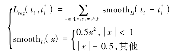
The formula is divided into two parts: the first part is the debris classification loss, the second part is the wear particle boundary regression loss. Where Pi is the predicted value of the translation and scaling parameter of the wear particle regression box; t * I is the offset of the actual target box corresponding to the wear particle prediction target box; lreg is the boundary regression loss, which is activated only when the area to be detected contains wear particles, i.e. p * I = 1; lreg uses the smoothliloss function, and the calculation formula is as follows: