
The relentless pursuit of quieter, more efficient, and more reliable power transmission systems is a cornerstone of modern mechanical engineering. In this endeavor, the helical gear stands as a workhorse, prized for its smooth operation and high load capacity compared to its spur gear counterpart. However, the theoretical perfection of the involute helicoidal surface, a line-contact geometry, often clashes with the realities of manufacturing imperfections, assembly errors, and elastic deformations under load. This mismatch is a primary source of vibration and noise, critical concerns in applications ranging from aerospace and marine propulsion to precision industrial machinery. To bridge this gap, gear modification, or “tooth flank correction,” has emerged as an essential design practice. I will explore in detail a sophisticated methodology for optimizing the tooth surface of helical gears, with the explicit goal of minimizing the amplitude of Loaded Transmission Error (LTE), thereby directly targeting the root cause of dynamic excitation.
The Imperative for Modification: From Theory to Practice
The standard involute helical gear is designed for conjugate action, theoretically ensuring a constant angular velocity ratio. In a perfect, rigid world, this results in zero transmission error. The transmission error (TE) is defined as the difference between the actual angular position of the driven gear and its theoretical position based on a perfect kinematic transfer from the driver. In reality, deflections under load cause deviations from this perfect path. The Loaded Transmission Error (LTE) is this deviation under operating conditions and is the primary dynamic excitation mechanism in gear systems. An LTE with large, discontinuous fluctuations creates significant vibratory forces and acoustic noise. The goal of optimization, therefore, is not to achieve zero LTE—an impossible feat—but to shape it into a smooth, low-amplitude function, ideally a straight line or a gentle curve with minimal fluctuation.
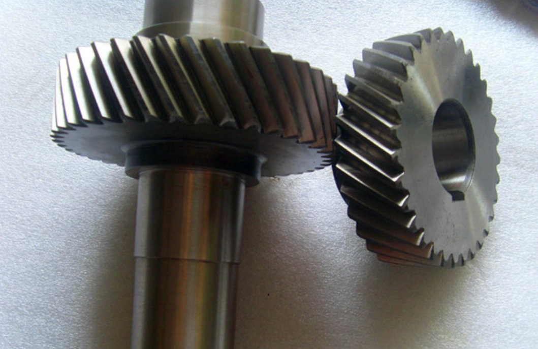
Unmodified helical gear pairs, while having a favorable contact ratio, are particularly sensitive to misalignment and load-induced deflections. Edge contacts, high-stress concentrations, and a load-dependent LTE amplitude are common issues. Modification strategically alters the microscopic geometry of the tooth flank from the theoretical design, introducing controlled deviations. These deviations, often mere micrometers in magnitude, are designed to compensate for expected deformations, ensuring a favorable contact pattern spreads evenly across the face width and tooth height under the designated load, thereby minimizing LTE fluctuations.
Constructing the Modified Helical Gear Flank
The foundation of any precise analysis is an accurate geometric model. Rather than defining the modified helical gear surface as a completely new entity, a robust approach is to construct it as a superposition of the theoretical involute helicoid and a “deviation surface” or “modification surface.” This method leverages the known perfect geometry and adds a corrective layer.
The theoretical flank of a helical gear can be represented by a vector function $\mathbf{R}_1(u_1, l_1)$, where $u_1$ and $l_1$ are the surface parameters (often related to the involute roll angle and the lead coordinate). Its corresponding unit normal vector is $\mathbf{n}_1(u_1, l_1)$.
The modification is typically defined in a domain convenient for specification and measurement: the rotated projection plane. In this plane, coordinates (x, y) relate to the theoretical flank coordinates $(R_x, R_y, R_z)$ as follows:
$$ x = \sqrt{R_x^2 + R_y^2}, \quad y = R_z $$
Modification curves are first defined in this 2D plane. For profile modification (along the tooth height), a common and effective design uses two parabolic segments and a straight (unmodified) zone in the center of the active profile. This is defined by four key parameters: the amount of tip relief ($y_1$), the amount of root relief ($y_3$), and the lengths of the relief zones at the tip ($y_4$) and root ($y_2$). Similarly, for lead modification (along the face width), a symmetric or asymmetric parabolic relief at the ends of the teeth can be defined, characterized by the relief amount at each end and the length of the unmodified central zone. Three-dimensional modification is then conceived as a combination (summation) of the profile and lead corrections.
To create a smooth, continuous deviation surface $\delta(x, y)$ from these piecewise curves, the rotated projection plane is discretized into an $m \times n$ grid. The modification amount $\delta’_{ij}$ is calculated at each grid node $(x_i, y_j)$ based on the defined curves. A bi-cubic B-spline surface is then fitted to this grid of data points. B-splines are chosen for their ability to create a smooth, $C^2$-continuous surface from local control points, perfectly representing the intended modification topology.
The final modified flank surface $\mathbf{R}_{1r}$ and its normal $\mathbf{n}_{1r}$ are then calculated by superimposing this deviation surface onto the theoretical flank:
$$ \mathbf{R}_{1r}(u_1, l_1) = \mathbf{R}_1(u_1, l_1) + \delta(u_1, l_1) \cdot \mathbf{n}_1(u_1, l_1) $$
$$ \mathbf{n}_{1r} = \left( \frac{\partial \mathbf{R}_1}{\partial u_1} + \frac{\partial \delta}{\partial u_1} \mathbf{n}_1 + \delta \frac{\partial \mathbf{n}_1}{\partial u_1} \right) \times \left( \frac{\partial \mathbf{R}_1}{\partial l_1} + \frac{\partial \delta}{\partial l_1} \mathbf{n}_1 + \delta \frac{\partial \mathbf{n}_1}{\partial l_1} \right) $$
The partial derivatives of $\delta$ with respect to the surface parameters $u_1$ and $l_1$ are obtained via the chain rule using the B-spline surface definition and the coordinate transformation. This formulation guarantees a kinematically correct and differentiable modified helical gear flank essential for subsequent contact analysis.
The Mathematical Core: Loaded Tooth Contact Analysis (LTCA)
Tooth Contact Analysis (TCA) simulates the meshing of gear flanks under no-load conditions, identifying the path of contact and unloaded transmission error. While vital, it is insufficient for predicting real-world behavior. Loaded Tooth Contact Analysis (LTCA) is the critical step that integrates mechanical compliance. It solves for the contact pressure distribution, loaded transmission error, and root stresses when the gears are subjected to operational torque.
The LTCA model treats the contact problem as a static elastic system. Under load, the teeth deflect, changing the theoretical point or line contact into a small elliptical contact area for each contacting pair. For computational efficiency in helical gear analysis, the instantaneous contact is often idealized as a line (the major axis of the contact ellipse) which is discretized into a series of nodes. When two or more tooth pairs are in contact simultaneously (due to the contact ratio), the system becomes a set of coupled elastic bodies.
The governing equations for LTCA are a set of compatibility and equilibrium conditions. For a two-pair contact instant, these can be expressed as:
1. Deformation Compatibility: The sum of the approach of the two gears at each contact point $j$ on pair $k$ must equal the rigid body approach $Z$ plus the initial separation (or flank error) $w_{jk}$ at that point.
$$ F_{jk} p_{jk} + w_{jk} = Z + d_{jk} \quad (k = I, II; \ j=1,…,n) $$
Here, $p_{jk}$ is the contact load at node $j$, $F_{jk}$ is the combined flexibility influence coefficient (relating load at $j$ to deflection at $j$ and other nodes, often compiled into a full flexibility matrix $\mathbf{F}_k$), and $d_{jk}$ is the final gap after loading.
2. Static Equilibrium: The sum of all contact loads across all contacting tooth pairs must equal the total applied normal load $P$.
$$ \sum_{j=1}^{n} p_{jI} + \sum_{j=1}^{n} p_{jII} = P $$
3. Non-Penetration Condition: Contact loads can only be positive (compressive), and a gap can only exist where the load is zero.
$$ d_{jk} = 0 \ \text{if} \ p_{jk} > 0; \quad d_{jk} \ge 0 \ \text{if} \ p_{jk} = 0 $$
This forms a constrained nonlinear programming problem. The flexibility matrix $\mathbf{F}$ is typically obtained through a detailed Finite Element Analysis (FEA) of a detailed gear sector model, capturing the bending, shearing, and contact deformations of the tooth and a portion of the gear body. The initial gap vector $\mathbf{w}$ comes directly from the TCA of the (modified) surfaces. Specialized algorithms, such as an improved Complex Method or quadratic programming solvers, are used to solve for the nodal loads $p_{jk}$, the body approach $Z$, and the gaps $d_{jk}$.
The crucial output, the Loaded Transmission Error (LTE) in angular arc-seconds, is derived from the rigid body approach $Z$:
$$ LTE = \frac{3600 \cdot Z \cdot R_{b2}}{\cos \beta_b} $$
where $R_{b2}$ is the base circle radius of the driven gear and $\beta_b$ is the base helix angle. The LTE is calculated over a full mesh cycle to obtain its functional form and, most importantly, its peak-to-peak amplitude $\Delta LTE$.
The Optimization Framework: Seeking the Minimum LTE Amplitude
The design challenge is to find the set of modification parameters (e.g., $y_1, y_2, y_3, y_4$ for profile modification) that yields the most favorable LTE curve. The formal optimization problem is established as follows:
Objective Function: Minimize the fluctuation of LTE amplitude across the expected load range. A weighted multi-load objective is prudent, as a gear rarely operates at a single torque.
$$ \min_{\mathbf{y}} \ F(\mathbf{y}) = w \left( \frac{\Delta LTE_1(\mathbf{y})}{\Delta LTE_{1,0}} \right) + (1-w) \left( \frac{\Delta LTE_2(\mathbf{y})}{\Delta LTE_{2,0}} \right) $$
Here, $\mathbf{y}$ is the vector of modification parameters, $\Delta LTE_1$ and $\Delta LTE_2$ are the LTE amplitudes at two designated load conditions (e.g., nominal and peak), and $\Delta LTE_{1,0}, \Delta LTE_{2,0}$ are the corresponding amplitudes for the unmodified gear pair. The weighting factor $w$ balances the importance of the two load cases. Normalizing by the unmodified amplitudes ensures a balanced optimization.
Design Variables ($\mathbf{y}$): These are the parameters defining the modification curves.
$$ \mathbf{y} = [y_1, y_2, y_3, y_4, …]^T $$
Constraints: Practical and manufacturable limits are imposed.
$$ \begin{aligned}
Q_{min} &\le y_1, y_3 \le Q_{max} \quad &\text{(relief amount bounds)} \\
L_{min} &\le y_2, y_4 \le L_{max} \quad &\text{(relief length bounds)} \\
|y_1 – y_3| &\le \Delta Q \quad &\text{(tip/root relief symmetry tolerance)} \\
|y_2 – y_4| &\le \Delta L \quad &\text{(relief zone length tolerance)}
\end{aligned} $$
The nature of this optimization problem is complex. The relationship between the modification parameters $\mathbf{y}$ and the objective function $F(\mathbf{y})$ is implicit and highly nonlinear. There is no analytical gradient; evaluating $F(\mathbf{y})$ requires a complete run of the geometric model construction, TCA, and LTCA for a given $\mathbf{y}$. Furthermore, the design space is likely multimodal, containing several local minima.
Therefore, a Genetic Algorithm (GA) is an excellent choice for the optimizer. GAs are population-based, stochastic search methods inspired by natural evolution. They operate on a coded representation of the parameters (chromosomes), evaluate a population of designs (fitness based on $F(\mathbf{y})$), and use selection, crossover, and mutation operators to evolve better solutions over generations. Their key advantages here are:
- Global Search Capability: Less prone to being trapped in poor local minima compared to gradient-based methods.
- Handles Discontinuous/Noisy Functions: Robust to the numerical noise inherent in the TCA/LTCA process.
- Works with Any Simulation: Only requires the ability to evaluate the objective function, not its derivatives.
The complete optimization workflow is as follows:
- Initialization: The GA creates an initial random population of design vectors $\mathbf{y}$ within the specified bounds.
- Analysis Loop: For each individual in the population:
- Construct the deviation surface $\delta(x,y)$ based on the parameters $\mathbf{y}$.
- Generate the modified helical gear flank $\mathbf{R}_{1r}(u_1, l_1)$.
- Perform TCA with the mating gear to find the unloaded contact path and initial gaps.
- Perform LTCA at the specified load cases to compute $\Delta LTE_1$ and $\Delta LTE_2$.
- Calculate the fitness score $F(\mathbf{y})$.
- Evolution: The GA performs selection, crossover, and mutation to produce a new generation of candidate solutions.
- Termination: Steps 2 and 3 repeat until a convergence criterion is met (e.g., maximum generations, stall in fitness improvement).
Application and Results: A Numerical Case Study
Consider a high-performance helical gear pair with the parameters listed below. The goal is to optimize the modification on the pinion (gear 1) to minimize LTE, with the gear (gear 2) remaining an unmodified theoretical involute.
| Parameter | Pinion (Gear 1) | Gear (Gear 2) |
|---|---|---|
| Number of Teeth, $z$ | 17 | 44 |
| Normal Module, $m_n$ (mm) | 6 | 6 |
| Normal Pressure Angle, $\alpha_n$ (°) | 20 | 20 |
| Helix Angle, $\beta$ (°) | 24.43 | 24.43 |
| Face Width, $w$ (mm) | 92 | 92 |
| Nominal Torque, $T_{nom}$ (Nm) | 800 | |
| Optimization Load Cases (Nm) | 500, 1000 (Weight: 0.4, 0.6) | |
The optimization is performed for three scenarios: profile modification only, lead modification only, and combined 3D modification. The design variable bounds are set as follows:
| Parameter | Profile Modification Bounds | Lead Modification Bounds |
|---|---|---|
| Relief Amount, $y_1, y_3$ (µm) | [10, 20] | [5, 15] |
| Unmodified/Relief Length, $y_2, y_4$ (mm) | [2, 3] | [60, 80] |
Using a GA with a population size of 20 and running for several generations (requiring ~60 full LTCA evaluations and about 5 minutes of computation time), the optimal parameters are found:
| Parameter | Optimal Profile Mod. | Optimal Lead Mod. | Optimal 3D Mod. (Profile) | Optimal 3D Mod. (Lead) |
|---|---|---|---|---|
| $y_1$ (µm) | 16.8 | 10 | 13 | 6 |
| $y_2$ (mm) | 2.62 | 75 | 2.17 | 78 |
| $y_3$ (µm) | 13.5 | 8 | 11 | 6 |
| $y_4$ (mm) | 2.68 | – | 2.2 | – |
The results are striking. The optimization successfully identifies modification parameters that significantly reduce the LTE amplitude at the nominal load (800 Nm) compared to the unmodified helical gear pair. Profile modification achieves a reduction of approximately 49%, lead modification 42%, and the combined 3D modification 47%. This demonstrates the potent effect of a carefully tailored flank correction.
A deeper analysis of the LTE behavior versus load reveals fundamental insights. For the unmodified helical gear, the contact pattern and overall contact ratio remain relatively constant with increasing load. Consequently, the LTE amplitude increases almost linearly with load due to the proportional increase in tooth deflection.
In contrast, the behavior of the modified helical gear is more complex and beneficial. At very low loads, the modification creates a slight initial separation, potentially reducing the contact ratio. As the load increases, the teeth deflect into contact, causing the operational contact ratio to increase gradually until full contact across the designed area is achieved. During this transition, the LTE amplitude may fluctuate. Once full contact is established under a sufficient “design load,” further increases in load cause the LTE amplitude to increase again, but at a much gentler, more stable rate than the unmodified gear. This is the hallmark of a well-optimized modification: it creates a load-insensitive, low-vibration state across the intended operating range.
Furthermore, Tooth Contact Analysis (TCA) of the optimized surfaces confirms excellent unloaded contact patterns. While lead-only modification can sometimes lead to edge contact under no-load conditions due to the crown, the 3D optimized modification consistently produces a centered, elliptical contact pattern that avoids edges, ensuring smooth engagement even during start-up or low-torque conditions.
Conclusion and Engineering Significance
The methodology detailed here—integrating precise geometric modeling of modified helical gear flanks, rigorous Loaded Tooth Contact Analysis, and robust global optimization via Genetic Algorithms—provides a powerful and systematic framework for designing high-performance, low-vibration helical gear transmissions. By directly targeting the minimization of Loaded Transmission Error amplitude, this approach attacks the core excitation mechanism for gear noise and vibration.
The key takeaways for the design engineer are:
- Precision Modeling is Non-Negotiable: Accurate representation of the modification as a smooth deviation surface superimposed on the theoretical involute is critical for predictive analysis.
- LTCA is the Essential Bridge: Only through Loaded Tooth Contact Analysis can the true functional performance, including load-sharing between teeth and the resulting LTE, be evaluated.
- Optimization is Multimodal and Implicit: The relationship between modification parameters and dynamic performance is complex, necessitating the use of global, non-gradient optimizers like Genetic Algorithms.
- Modification Changes Load-Dependent Behavior: A well-designed modification for a helical gear not only reduces LTE at a specific load but, more importantly, creates a stable, high-contact-ratio condition that makes performance less sensitive to load variations.
This approach is universally applicable, extending beyond the parabolic profile and lead corrections shown here. It can incorporate more complex modification topographies, account for manufacturing and alignment errors in the optimization loop, and be adapted for other gear types like double helical gears or spiral bevel gears. In the relentless pursuit of mechanical harmony, such computational design and optimization tools are indispensable for pushing the boundaries of efficiency, reliability, and quiet operation in power transmission systems dominated by the versatile helical gear.