
I study the nonlinear vibration and chaotic behavior of a six-degree-of-freedom helical gear transmission system, and I design neural-network controllers that can drive the system from irregular motion into a desired periodic orbit. The helical gear pair is a central component in high-speed train gearboxes, and its dynamic behavior directly affects operational safety, acoustic comfort, and fatigue life. Because a helical gear pair is subjected to time-varying mesh stiffness, transmission error, backlash, damping, support flexibility, and external load fluctuations, its response can include periodic motion, multi-periodic motion, quasi-periodic motion, and chaos. I focus on how these nonlinear effects shape the bifurcation structure of the helical gear system and how a radial basis function neural network controller, optimized by an improved gravitational search algorithm, can suppress chaotic vibration.
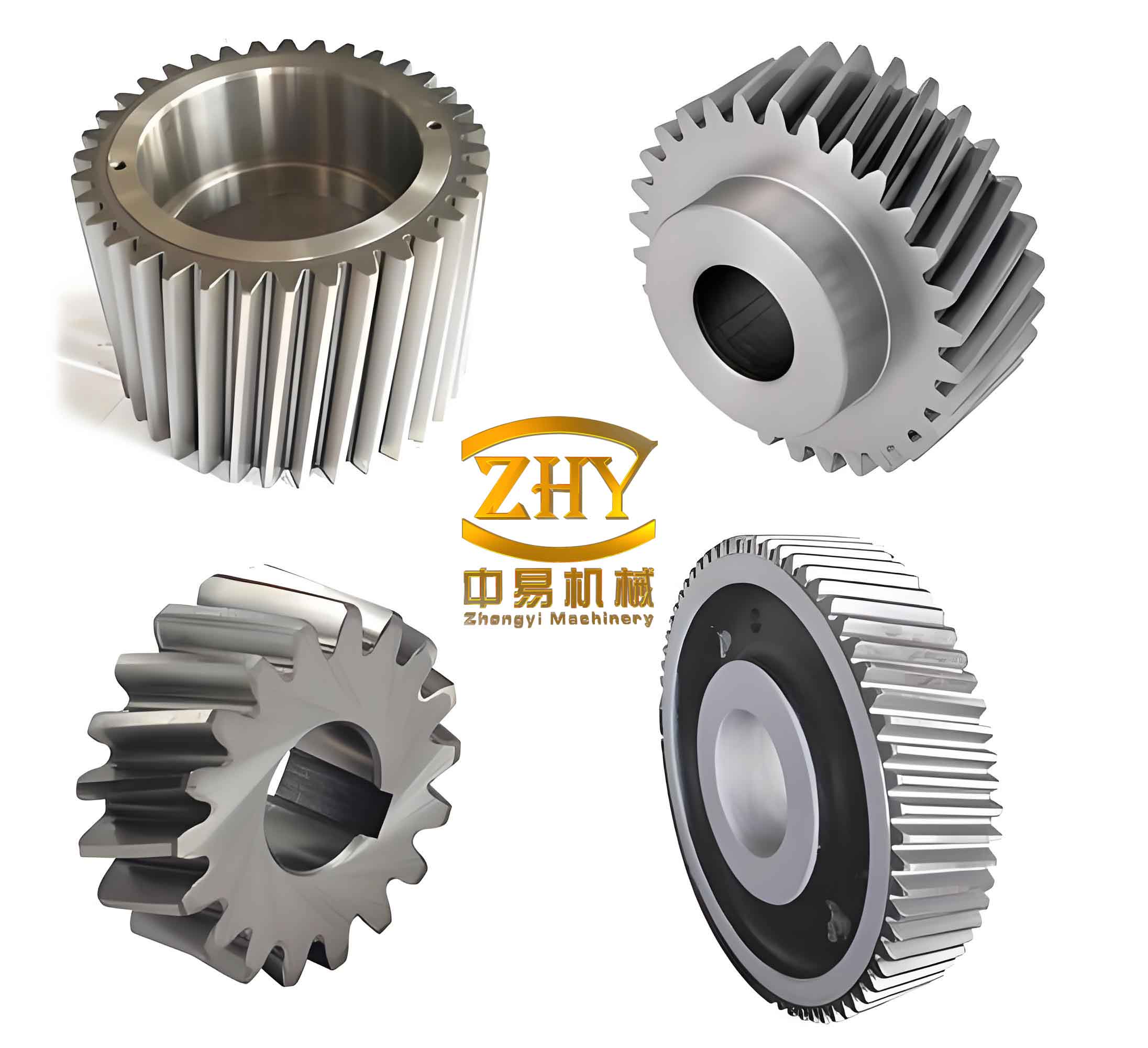
1. Motivation and scope
When a helical gear pair operates under varying speed and load, the contact ratio changes, the mesh stiffness fluctuates, and the loaded transmission error excites internal vibration. A small change in meshing frequency or load coefficient can move the helical gear system from a stable periodic state into a chaotic state. In a train gearbox, such chaotic vibration may increase dynamic load, accelerate tooth-surface wear, produce strong noise, and reduce the reliability of the whole transmission chain. Therefore, I model the helical gear system, identify the parameter regions where chaos appears, and design controllers that apply small perturbations to controllable parameters.
The main contributions I present are as follows. I establish a six-degree-of-freedom dynamic model of a helical gear pair using the concentrated-mass method. I derive the dimensionless state equations and solve them with a fourth-to-fifth order Runge–Kutta method. I analyze the influence of time-varying mesh stiffness, transmission error, and backlash through two-parameter diagrams. I determine bifurcation intervals for meshing frequency and load coefficient. I design a radial basis function neural network controller and a back-propagation neural network controller for comparison. I improve the gravitational search algorithm through Sobol initialization, particle memory, adaptive decay, weighted inertial mass, and chaotic search. Finally, I apply the controllers to chaotic, quasi-periodic, and multi-periodic helical gear motions and compare their performance.
2. Six-degree-of-freedom helical gear model
I use the concentrated-mass method for a helical gear pair. The two gears have equivalent masses \(m_1\) and \(m_2\), rotary inertias \(I_1\) and \(I_2\), angular displacements \(\theta_1\) and \(\theta_2\), torques \(T_1\) and \(T_2\), support stiffnesses \(k_{iy}\) and \(k_{iz}\), support dampings \(c_{iy}\) and \(c_{iz}\), radial preloads \(F_{bi}\), time-varying mesh stiffness \(K_h(t)\), mesh damping \(C_h\), and comprehensive transmission error \(e(t)\). The model includes two transverse directions and one torsional direction for each gear, giving six degrees of freedom.
The relative displacement along the line of action is written as
$$ p=(Y_1-Y_2)\sin\beta+(Z_1-Z_2)\cos\beta+r_1\theta_1-r_2\theta_2-e(t), $$
where \(Y_i\) and \(Z_i\) are transverse displacements, \(r_i\) are base radii, and \(\beta\) is the helix angle. The dynamic mesh force is
$$ F_n=K_h(t)f(p)+C_h\dot{p}, $$
where \(f(p)\) is the backlash function. The transverse force components are
$$ F_y=F_n\cos\beta,\qquad F_z=F_n\sin\beta. $$
Applying Newton’s second law gives the dimensional equations of motion:
$$ \begin{aligned} m_1\ddot{Y}_1+C_{1y}\dot{Y}_1+k_{1y}Y_1 &= F_{b1}, \\ m_1\ddot{Z}_1+C_{1z}\dot{Z}_1+k_{1z}Z_1 &= F_{b1}, \\ I_1\ddot{\theta}_1 &= T_1-F_n r_1, \\ m_2\ddot{Y}_2+C_{2y}\dot{Y}_2+k_{2y}Y_2 &= -F_{b2}, \\ m_2\ddot{Z}_2+C_{2z}\dot{Z}_2+k_{2z}Z_2 &= -F_{b2}, \\ I_2\ddot{\theta}_2 &= -T_2+F_n r_2. \end{aligned} $$
After dimensionless treatment, I define the dimensionless time \(\tau=\Omega_n t\), the dimensionless meshing frequency \(\Omega=\Omega_h/\Omega_n\), damping ratios \(\zeta_{ij}=c_{ij}/(2m_j\Omega_n)\), stiffness ratios \(\kappa_{ij}=k_{ij}/(m_j\Omega_n^2)\), load coefficients \(f_{pm}\) and \(f_{pv}\), and transmission-error excitation \(f_e\). The dimensionless state vector is
$$ \mathbf{x}=[x_1,x_2,x_3,x_4,x_5,x_6,x_7,x_8,x_9,x_{10}]^T, $$
where \(x_1,x_3,x_5,x_7\) are displacement coordinates, \(x_2,x_4,x_6,x_8\) are their velocities, \(x_9=p\), and \(x_{10}=\dot{p}\). The state equation has the general form
$$ \dot{\mathbf{x}}=\mathbf{f}(\mathbf{x},\tau;\Omega,\varepsilon,f_{pm},f_{pv},b), $$
and its components include the support forces, mesh force, backlash function, and transmission-error excitation. The dimensionless mesh stiffness is
$$ k_h(\tau)=1+\varepsilon\cos(\Omega\tau), $$
where \(\varepsilon\) is the stiffness amplitude coefficient. The dimensionless backlash function is
$$ f(x_9,b)= \begin{cases} x_9-b, & x_9>b, \\ 0, & |x_9|\le b, \\ x_9+b, & x_9<-b. \end{cases} $$
I use the following gear-pair parameters in the numerical study.
| Quantity | Symbol | Value |
|---|---|---|
| Number of teeth | \(z_1/z_2\) | 29/69 |
| Normal module | \(m_n\) | 7 mm |
| Pressure angle | \(\alpha\) | 26° |
| Helix angle | \(\beta\) | 20° |
| Normal profile shift | \(x_1/x_2\) | 0/-0.285 |
| Center distance | \(a\) | 363 mm |
| Face width | \(B_1/B_2\) | 75/70 mm |
3. Nonlinear factors in the helical gear system
The principal nonlinear factors I consider are time-varying mesh stiffness, comprehensive transmission error, and backlash. The time-varying mesh stiffness of a helical gear pair changes periodically as the number of contacting tooth pairs alternates. I represent it by a Fourier series, and in the numerical model I retain the fundamental harmonic:
$$ K_h(t)=K_m\left[1+\varepsilon\cos\left(\frac{2\pi t}{T}\right)\right]. $$
The comprehensive transmission error consists of design transmission error and manufacturing transmission error:
$$ e(t)=e_{\delta}(t)+e_{\Delta}(t). $$
The backlash function introduces piecewise stiffness and possible contact loss. I classify the contact state through the minimum mesh error \(x_{\min}\) and half backlash \(b\):
$$ \text{impact}= \begin{cases} 0, & x_{\min}>b, \\ 1, & x_{\min}=b, \\ 2, & x_{\min}<-b. \end{cases} $$
I also use the contact-loss duty ratio \(DC_1\), back-side mesh ratio \(DC_2\), and dynamic load coefficient \(DLC\):
$$ DC_1=\frac{t_1}{T},\qquad DC_2=\frac{t_2}{T}, $$
$$ DLC=\frac{1}{\sum_{i=1}^{3}k_i}\max\left(\sum_{i=1}^{3}k_i f(x_i,b),\sum_{i=1}^{3}\zeta_i x_i\right). $$
These quantities help me judge whether the helical gear pair is transmitting motion smoothly or is experiencing impact, separation, or back-side contact.
4. Dynamic analysis tools
I use several tools to identify the motion state of the helical gear system. A phase portrait shows whether the trajectory is a closed curve or a dense set of curves. A bifurcation diagram shows how the number of solution branches changes with a parameter. A Lyapunov exponent diagram gives a quantitative indicator of chaos. A Poincaré section reduces a continuous trajectory to a discrete map and distinguishes periodic, quasi-periodic, and chaotic motion.
| Tool | Interpretation |
|---|---|
| Phase portrait | Closed curve: periodic; multiple curves: multi-periodic; dense curves: quasi-periodic or chaotic. |
| Bifurcation diagram | One point: period-one; two points: period-two; dense points: chaos or quasi-periodicity. |
| Lyapunov exponent | \(\lambda<0\): stable; \(\lambda=0\): marginal; \(\lambda>0\): chaotic. |
| Poincaré section | Finite points: periodic; closed curve: quasi-periodic; scattered cloud: chaotic. |
The largest Lyapunov exponent is approximated by
$$ \lambda_{\max}=\lim_{n\to\infty}\frac{1}{n}\sum_{i=0}^{n-1}\ln\left|\frac{df}{dx}(x_i,\mu)\right|. $$
For the helical gear model, I compute the Poincaré section by sampling the state once per mesh period. The distance between two successive Poincaré points becomes the key control input.
5. Effects of nonlinear parameters on helical gear dynamics
I first examine the influence of time-varying mesh stiffness. I compare two cases, \(\varepsilon=0.1\) and \(\varepsilon=0.25\), while keeping the other parameters fixed. The two-parameter diagrams show that when \(\varepsilon\) increases, the chaotic region of the helical gear system decreases significantly, while the periodic region expands. The no-impact region also increases. This means that a larger mesh-stiffness amplitude can enrich the periodic behavior of the helical gear pair and reduce impact severity.
| Quantity | \(\varepsilon=0.1\) | \(\varepsilon=0.25\) | Trend |
|---|---|---|---|
| Chaotic area | 49.6% | 9.0% | Decreases |
| No-impact area | 2.4% | 5.4% | Increases |
| Period-2 area | Baseline | +18% | Increases |
| Period-4 area | Baseline | +1.9% | Increases |
| Period-8 area | Baseline | +6.5% | Increases |
I then examine comprehensive transmission error. I compare \(f_e=0.01\) and \(f_e=0.05\). As transmission error increases, the chaotic region of the helical gear system becomes much larger, and the periodic region shrinks. The contact-loss duty ratio also increases, which indicates worse motion stability. The dynamic load coefficient rises, meaning that the tooth root and tooth surface experience stronger alternating load.
| Motion state | \(f_e=0.01\) | \(f_e=0.05\) | Interpretation |
|---|---|---|---|
| Period-one with single-sided impact | 32.5% | 35.8% | Slightly increases |
| Period-two with single-sided impact | 35.4% | 13.0% | Decreases |
| Period-4/8/16 | 17.6% | 1.1% | Strongly decreases |
| Chaos | 9.0% | 50.4% | Strongly increases |
Finally, I examine backlash. I compare \(b=0.014\) and \(b=1\). When backlash is very small, back-side contact and double-sided impact can appear. When backlash increases, the double-sided impact region disappears. However, the single-sided impact chaotic region can grow. Thus, backlash has a strong influence on the back-side mesh ratio and on impact type, and an extremely small backlash is not always beneficial for a helical gear pair.
| Quantity | \(b=0.014\) | \(b=1\) | Trend |
|---|---|---|---|
| Double-sided impact area | 17.5% | 0% | Disappears |
| Period-2 area | 31.8% | 35.4% | Increases |
| Period-4/8/16 area | 9.2% | 17.6% | Increases |
| Back-side mesh ratio | Nonzero | Zero | Reduced |
From these comparisons, I conclude that increasing mesh stiffness can improve the smoothness of the helical gear transmission, an excessively large transmission error intensifies separation and vibration, and an excessively small backlash aggravates back-side meshing.
6. Bifurcation and chaos intervals
I select the meshing frequency \(\Omega\) as the main bifurcation parameter. For one parameter set, the helical gear system behaves as follows. For \(\Omega\in[1.15,1.173]\), the motion is period-one. Around \(\Omega=1.173\), a saddle-node bifurcation occurs, and the helical gear motion becomes period-two. For \(\Omega\in[1.173,1.2338]\), the motion remains period-two. Near \(\Omega=1.2327\), period-doubling begins, and the helical gear system passes through period-four and period-eight before entering chaos. For \(\Omega\in[1.236,1.336]\), the motion is chaotic with periodic windows. After \(\Omega=1.339\), inverse period-doubling appears, and the helical gear system returns to period-eight, period-four, period-two, and finally period-one.
| Parameter interval | Motion state | Bifurcation feature |
|---|---|---|
| \(\Omega\in[1.15,1.173]\) | Period-one | Stable periodic orbit |
| \(\Omega\approx1.173\) | Period-two | Saddle-node bifurcation |
| \(\Omega\in[1.173,1.2338]\) | Period-two | Stable period-two |
| \(\Omega\approx1.2327\) | Period-four/eight | Period-doubling |
| \(\Omega\in[1.236,1.336]\) | Chaos | Chaotic band with windows |
| \(\Omega>1.339\) | Period-eight to period-one | Inverse period-doubling |
I also choose the load coefficient \(f_{pm}\) as a bifurcation parameter. The helical gear system follows a route of period-one, period-two, and chaos, followed by inverse period-doubling back to period-four, period-two, and period-one. This confirms that the load coefficient is a suitable control parameter for suppressing chaos in the helical gear system.
In the \(\Omega\)-\(f_{pm}\) plane, I identify both chaotic and periodic regions. Some chaotic regions can be driven to periodic motion by perturbing only one parameter, but other regions require simultaneous perturbation of both meshing frequency and load coefficient. This observation motivates the two-input, two-output controller design that I later develop.
7. Radial basis function neural network controller
I use a radial basis function neural network as the core of the controller because it can approximate a nonlinear mapping with a compact structure. The network has an input layer, a hidden layer, and an output layer. The hidden layer uses Gaussian radial basis functions:
$$ \phi_j(r)=\exp\left(-\frac{r^2}{2b_j^2}\right), $$
where \(r=\|\mathbf{x}-\mathbf{c}_j\|\) is the Euclidean distance from the input vector to the \(j\)-th center \(\mathbf{c}_j\), and \(b_j\) is the width. The output is
$$ y=\sum_{j=1}^{5}\omega_j\phi_j(\|\mathbf{x}-\mathbf{c}_j\|). $$
I choose a 2-5-1 structure for single-parameter control: two inputs, five hidden neurons, and one output. The inputs are the distances between successive Poincaré points:
$$ D(k)=[d(k-1),d(k)], $$
$$ d(k)=\|X(k)-X(k-1)\|. $$
The output \(u(k)\) is the perturbation applied to a controllable parameter, such as meshing frequency or load coefficient. I limit the perturbation by
$$ |u(k)|\le u^*. $$
If the computed perturbation exceeds the limit, I set \(u(k)=0\) for that control cycle. The control objective is to make the distance between successive Poincaré points approach a desired value \(d^*\):
$$ d^*=\text{eps}\approx 2.2204\times10^{-16}. $$
For comparison, I also design a back-propagation neural network controller with a 2-5-1 structure. Its activation function is the sigmoid function:
$$ f(x)=\frac{1}{1+e^{-x}}. $$
The weighted sum in the hidden layer is
$$ h_j=f\left(\sum_{i=1}^{2}w_{ij}D_i+b_j\right), $$
and the output is
$$ u=f\left(\sum_{j=1}^{5}v_jh_j+c\right). $$
The controller parameters are not trained from a large data set. Instead, I optimize them with an improved gravitational search algorithm. This avoids the need for a highly accurate analytical model of the helical gear system and also avoids online training.
| Controller | Structure | Activation or basis | Optimized parameters |
|---|---|---|---|
| RBF neural network | 2-5-1 | Gaussian function | Output weights, centers, widths |
| BP neural network | 2-5-1 | Sigmoid function | Hidden-to-output weights and biases |
8. Fitness function and control flow
The fitness function links the improved gravitational search algorithm to the neural network controller. I define it as the accumulated error between the actual Poincaré distance and the desired distance:
$$ fit(P_i)=\sum_{k=1}^{L}\left|\,\|X(k)-X(k-1)\|-d^*\,\right|. $$
A smaller fitness value means that the controller drives the helical gear motion closer to a fixed point on the Poincaré section, which corresponds to a periodic orbit. The control flow is as follows.
| Step | Operation |
|---|---|
| 1 | Iterate the helical gear system for 200 cycles to obtain the uncontrolled Poincaré points. |
| 2 | Compute the initial distance \(D_0\) from the last three Poincaré points. |
| 3 | Initialize the improved gravitational search algorithm. |
| 4 | Pass each particle position as a candidate controller parameter set. |
| 5 | Apply the controller output \(u(k)\) to the chosen parameter. |
| 6 | Check the perturbation limit; if exceeded, set \(u(k)=0\). |
| 7 | Compute new Poincaré distances and evaluate the fitness. |
| 8 | Update particle positions until the maximum iteration is reached. |
| 9 | Output the best controller parameters and the controlled periodic orbit. |
9. Improved gravitational search algorithm
The standard gravitational search algorithm treats each candidate solution as a particle with mass. The inertial mass is computed from the fitness value:
$$ m_i(t)=\frac{fit_i(t)-worst(t)}{best(t)-worst(t)}, $$
$$ M_i(t)=\frac{m_i(t)}{\sum_{j=1}^{N}m_j(t)}. $$
The attractive force between particles \(i\) and \(j\) in dimension \(d\) is
$$ F_{ij}^d(t)=G(t)\frac{M_i(t)M_j(t)}{R_{ij}(t)+\varepsilon}\left(x_j^d(t)-x_i^d(t)\right), $$
where \(R_{ij}(t)\) is the Euclidean distance between particles and \(\varepsilon\) is a small constant. The gravitational constant is
$$ G(t)=G_0e^{-\alpha t/T}. $$
The acceleration, velocity, and position updates are
$$ a_i^d(t)=\frac{F_i^d(t)}{M_i(t)}, $$
$$ v_i^d(t+1)=rand_i\,v_i^d(t)+a_i^d(t), $$
$$ x_i^d(t+1)=x_i^d(t)+v_i^d(t+1). $$
The standard algorithm has strong global search ability but weak local exploitation, and it can fall into a local optimum. I improve it in five ways.
9.1 Sobol initialization
I initialize the particle population with a Sobol sequence rather than a pseudo-random sequence. The Sobol sequence distributes initial points more uniformly in the search space. This improves the diversity of the initial helical gear controller parameters and increases the probability of finding the global optimum.
9.2 Particle memory
I introduce memory terms similar to those in particle swarm optimization. The velocity update becomes
$$ V(t+1)=rand_1V(t)+a+c_1rand_2(qbest-X)+c_2rand_3(gbest-X), $$
where \(qbest\) is the individual memory, \(gbest\) is the global best, and
$$ c_1=\left(1-\frac{t}{T}\right)^{\sigma},\qquad c_2=\left(1+\frac{t}{T}\right)^{\sigma}. $$
This makes the early stage favor global exploration and the later stage favor convergence toward the best region.
9.3 Adaptive decay factor
I use an adaptive decay factor so that the gravitational constant decreases smoothly with iteration:
$$ \alpha(t)=\alpha_0\exp\left(\frac{t}{T}\ln 10\right). $$
This allows larger steps in the early search and smaller steps near the optimum, reducing oscillation around the best solution.
9.4 Weighted inertial mass
I add a weight to the inertial mass to amplify differences among particles:
$$ MG_i(t)=M_i(t)\left(1+\frac{10}{\ln(t)+1}\right). $$
I also adjust non-best fitness values by a random factor to avoid premature convergence when several particles have similar fitness:
$$ fitg_i(t)=rand(t)\,fit_i(t). $$
9.5 Chaotic search
In the late stage, I perform a chaotic search around the current global best \(Lbest\). I use the piecewise chaotic map:
$$ x(t+1)= \begin{cases} \dfrac{x(t)}{p}, & 0\le x(t)<p, $$="" &="" 0.5\le="" 1-p\le="" <p="" \\[6pt]="" \dfrac{1-x(t)-p}{0.5-p},="" \dfrac{1-x(t)}{p},="" \dfrac{x(t)-p}{0.5-p},="" \end{cases}="" p\le="" x(t)<0.5,="" x(t)<1-p,="" x(t)The chaotic search generates candidate points in a local neighborhood and improves the precision of the controller parameters. This is important because a chaotic helical gear system is highly sensitive to small perturbations.
| Improvement | Purpose | Effect |
|---|---|---|
| Sobol initialization | Better coverage of search space | Higher diversity |
| Particle memory | Avoid local optima | Better convergence path |
| Adaptive decay | Balance exploration and exploitation | Smaller oscillation |
| Weighted inertial mass | Amplify particle differences | Faster movement to best region |
| Chaotic search | Improve local precision | Higher accuracy |
I validate the improved algorithm with five multimodal test functions.
| Function | Expression | Range |
|---|---|---|
| Griewank | \(\displaystyle f(x)=\frac{1}{4000}\sum_{i=1}^{N}x_i^2-\prod_{i=1}^{N}\cos\left(\frac{x_i}{\sqrt{i}}\right)+1\) | \([-600,600]^n\) |
| Rastrigin | \(\displaystyle f(x)=10N+\sum_{i=1}^{N}\left[x_i^2-10\cos(2\pi x_i)\right]\) | \([-5,5]^n\) |
| Ackley | \(\displaystyle f(x)=-a\exp\left(-b\sqrt{\frac{1}{N}\sum x_i^2}\right)-\exp\left(\frac{1}{N}\sum\cos(cx_i)\right)+a+\exp(1)\) | \([-32,32]^n\) |
| Schaffer | \(\displaystyle f(x)=0.5+\frac{0.5+(\sum x_i^2)^2-0.5}{(1+0.001\sum x_i^2)^2}\) | \([-100,100]^n\) |
| Alpine | \(\displaystyle f(x)=\sum_{i=1}^{N}|x_i\sin x_i+0.1x_i|\) | \([-10,10]^n\) |
The tests show that the improved gravitational search algorithm escapes local optima more often and reaches higher precision than the standard algorithm. I therefore use it to optimize the RBF and BP controller parameters for the helical gear system.
10. Chaos control in the inverse period-doubling interval
I select a chaotic case in the inverse period-doubling interval, with \(\Omega=1.31\). The uncontrolled phase portrait contains multiple curves, and the Poincaré section contains many scattered points. I apply the RBF and BP neural network controllers to perturb the meshing frequency. The control results are summarized below.
| Target motion | RBF control speed | BP control speed | Perturbation comparison |
|---|---|---|---|
| Period-one | Fast, about 40 cycles | Fast, about 40 cycles | Similar after stabilization |
| Period-two | Fast, about 40 cycles | Fast, about 40 cycles | RBF larger in one case |
| Period-four | Fast, about 5 control cycles | Fast, about 5 control cycles | RBF smaller |
| Period-sixteen | Comparable | Comparable | Comparable |
For the inverse period-doubling interval, the two controllers achieve similar control speed and similar target orbits. The RBF controller sometimes uses a larger perturbation, but after the helical gear system reaches the periodic orbit, the perturbation becomes nearly constant. The controller parameters are optimized offline by the improved gravitational search algorithm, so no online training is needed.
11. Chaos control in the saddle-node bifurcation interval
I choose \(\Omega=1.25\), where the helical gear system is chaotic after a saddle-node bifurcation. The phase portrait contains many trajectories, and the Poincaré section is scattered. I apply continuous small perturbations to the meshing frequency. The RBF controller drives the helical gear system to period-one within about 40 control cycles. The BP controller also drives the system to period-one, but its perturbation range is larger. Therefore, for the saddle-node bifurcation interval, the RBF controller has better performance.
| Controller | Target | Control cycles | Perturbation range | Performance |
|---|---|---|---|---|
| RBF | Period-one | About 40 | Smaller | Better |
| BP | Period-one | About 40 | Larger | Good |
12. Control of multi-periodic helical gear motion
I choose a multi-periodic case near \(\Omega=1.338\). The phase portrait has several closed curves, and the Poincaré section has a finite set of points. I use the controllers to drive the helical gear motion to period-one, period-two, and period-four.
| Initial motion | Target | RBF performance | BP performance |
|---|---|---|---|
| Multi-periodic | Period-one | About 10 cycles, smaller perturbation | About 20 cycles, larger perturbation |
| Multi-periodic | Period-two | About 10 cycles, larger perturbation | About 10 cycles, smaller perturbation |
| Multi-periodic | Period-four | About 10 cycles, smaller perturbation | About 10 cycles, larger perturbation |
| Period-four | Period-one | About 10 cycles, larger perturbation | About 10 cycles, smaller perturbation |
| Period-four | Period-two | About 10 cycles, larger perturbation | About 10 cycles, smaller perturbation |
For multi-periodic motion, both controllers are effective. The RBF controller is faster in the period-one control case, while the BP controller sometimes requires a smaller perturbation. Overall, the two controllers are comparable in this interval, but the RBF controller is more consistent across different target orbits.
13. Control of quasi-periodic helical gear motion
I choose a quasi-periodic case with \(\Omega=1.93\). The phase portrait contains many closed curves, the Poincaré section is a closed curve, and the time history is irregular. I apply the RBF and BP controllers to drive the quasi-periodic helical gear motion to period-one and period-three.
| Target | RBF control cycles | BP control cycles | Perturbation | Better controller |
|---|---|---|---|---|
| Period-one | About 40 | About 60 | Similar | RBF |
| Period-three | Fast | Slower | RBF larger | RBF |
The RBF controller converges faster for quasi-periodic motion. The BP controller eventually reaches a similar periodic orbit, but it needs more control cycles. This shows that the RBF controller is more suitable for quasi-periodic helical gear vibration, where the Poincaré section is a closed curve rather than a finite point set.
14. Chaos control using the load coefficient
I select \(f_{pm}=0.011\), where the helical gear system is chaotic under load variation. I use the load coefficient as the control parameter and drive the system to period-one, period-two, and period-four.
| Target | RBF perturbation | BP perturbation | Target orbit | Performance |
|---|---|---|---|---|
| Period-one | Smaller | Larger | Different orbits | RBF better |
| Period-two | Similar | Similar | Same orbit | Comparable |
| Period-four | Similar | Similar | Same orbit | Comparable |
When the load coefficient is the control parameter, both controllers can suppress chaos. For period-one control, the RBF controller requires a smaller load perturbation. For period-two and period-four control, the two controllers perform similarly. This confirms that the RBF controller is not restricted to one control parameter and can handle different controllable variables in the helical gear system.
15. Simultaneous control of meshing frequency and load coefficient
Some chaotic and quasi-periodic regions in the \(\Omega\)-\(f_{pm}\) plane cannot be controlled effectively by perturbing only one parameter. I therefore design a parallel RBF controller with two RBF networks. One network outputs the meshing-frequency perturbation \(R(k)\), and the other outputs the load-coefficient perturbation \(F(k)\). The controller has two inputs, \(D(k-1)\) and \(D(k)\), and two outputs, \(R(k)\) and \(F(k)\).
| Initial region | Target region | Controlled motion | Output 1 | Output 2 |
|---|---|---|---|---|
| Chaotic \(K_1\) | Periodic \(K_2\) | Period-one | Meshing-frequency perturbation | Load perturbation |
| Chaotic \(K_3\) | Periodic \(K_4\) | Period-two | Small | Stabilized |
| Chaotic \(K_5\) | Periodic \(K_6\) | Period-four | Active | Active |
The parallel RBF controller drives the helical gear system from chaotic and quasi-periodic motion to period-one, period-two, and period-four. In some cases, the perturbation of one parameter becomes nearly zero after the system reaches the target orbit, while the other parameter remains slightly adjusted. In other cases, both perturbations remain active. This demonstrates that the parallel RBF controller can handle multi-parameter control and is more flexible than a single-parameter controller.
16. Summary of control performance
I compare the RBF and BP controllers across several helical gear motion types.
| Motion type | Control parameter | RBF performance | BP performance | Preferred controller |
|---|---|---|---|---|
| Inverse period-doubling chaos | \(\Omega\) | Good | Good | Comparable |
| Saddle-node chaos | \(\Omega\) | Smaller perturbation | Larger perturbation | RBF |
| Multi-periodic motion | \(\Omega\) | Faster in some targets | Smaller perturbation in some targets | Comparable |
| Quasi-periodic motion | \(\Omega\) | Faster convergence | Slower convergence | RBF |
| Load chaos | \(f_{pm}\) | Smaller perturbation for period-one | Larger for period-one | RBF |
| Two-parameter chaos | \(\Omega,f_{pm}\) | Effective | Not used | RBF parallel |
The RBF controller has several advantages for the helical gear system. It does not require the Jacobian matrix of the system. It does not require a highly accurate analytical model. It can be optimized offline by the improved gravitational search algorithm. It can drive chaotic, quasi-periodic, and multi-periodic helical gear motion into a desired periodic orbit using only small perturbations. The improved gravitational search algorithm increases the probability of finding a high-quality controller parameter set, which is essential because the chaotic helical gear system is sensitive to perturbations.
17. Conclusions
I established a six-degree-of-freedom dynamic model of a helical gear transmission system and analyzed its nonlinear vibration under time-varying mesh stiffness, comprehensive transmission error, and backlash. The main conclusions are as follows.
First, the time-varying mesh stiffness strongly affects the bifurcation structure of the helical gear system. A larger stiffness amplitude reduces the chaotic area and increases the periodic area and the no-impact area. This tends to make the helical gear transmission smoother.
Second, a larger comprehensive transmission error increases the chaotic area, the contact-loss duty ratio, and the dynamic load coefficient. Therefore, improving manufacturing and assembly accuracy is beneficial for reducing helical gear vibration.
Third, backlash has a strong influence on back-side meshing. A very small backlash can increase double-sided impact and back-side contact, while a larger backlash removes double-sided impact but may enlarge the single-sided chaotic region.
Fourth, the meshing frequency and load coefficient are suitable control parameters. The helical gear system exhibits saddle-node bifurcation, period-doubling, inverse period-doubling, quasi-periodic motion, and chaos over different parameter intervals.
Fifth, the improved gravitational search algorithm combines Sobol initialization, particle memory, adaptive decay, weighted inertial mass, and chaotic search. It performs better than the standard algorithm on multimodal test functions and provides reliable controller parameters.
Sixth, the RBF neural network controller effectively suppresses chaos in the helical gear system. It performs better than the BP controller in saddle-node chaos, quasi-periodic motion, and load-induced chaos. For inverse period-doubling chaos and multi-periodic motion, the two controllers are comparable. The parallel RBF controller can simultaneously perturb meshing frequency and load coefficient, which extends the controllable region of the helical gear system.
In future work, I plan to include more nonlinear factors such as friction, thermal deformation, bearing clearance, and time-varying support stiffness in the helical gear model. I also plan to carry out experimental validation so that the control strategy can be evaluated under realistic gearbox operating conditions. The results I obtained provide a theoretical basis for avoiding chaotic vibration and improving the operational reliability of helical gear transmission systems.