
In this study I investigate the surge mechanism of a helical gear pair operating under oil lubrication, with particular attention to solid-liquid interfacial slip and meshing impact. I treat surge not as a purely aerodynamic phenomenon but as a coupled lubrication-dynamics instability in which the oil film between mating helical gear teeth undergoes abrupt thickening, repeated oscillation, and partial backflow. The central aim is to construct a mathematical model of helical gear surge, to couple it with the dynamic model of a helical gear pair, and to identify parameters that may suppress surge and improve transmission stability.
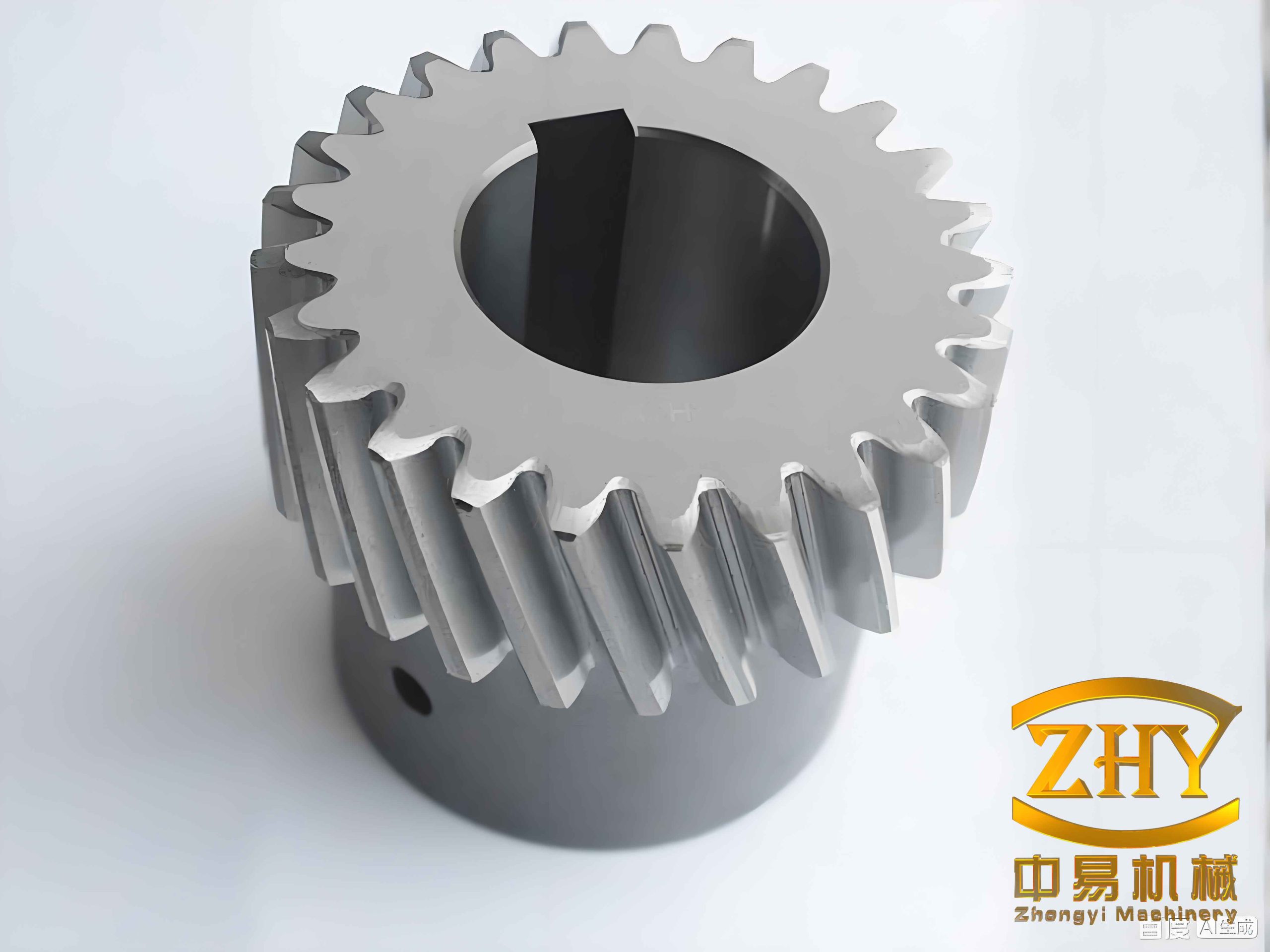
I begin with the observation that a helical gear transmission system always contains manufacturing errors, assembly errors, tooth surface deviations, and time-varying contact conditions. Under high speed and heavy load, the mating teeth do not enter contact in a perfectly smooth manner. A relative base pitch error is produced by the deflection of the previous tooth pair, and the following tooth pair may contact prematurely. This premature contact creates a meshing impact, a sudden change in entrainment velocity, and a transient disturbance in the oil film. When the oil supply cannot respond quickly enough, the lubricant between the two tooth surfaces may be entrained, expelled, and partially returned. This returned flow is the necessary condition for helical gear surge. The consequences include increased wear, reduced service life, alternating stress, fatigue damage, crack initiation, strong vibration, and noise.
To describe the problem consistently, I define the helical gear surge state through the following physical conditions: a meshing impact occurs; the interfacial shear stress exceeds a limiting value; interfacial slip appears near the solid surfaces; a backflow component develops in the lubricant film; and the central film thickness shows a sudden increase followed by low-frequency oscillation. The helical gear pair therefore behaves as a nonlinear fluid-solid system in which the lubricant film, the tooth contact, and the rotational motion interact.
The geometric and operating parameters used in my analysis are summarized in Table 1. These values provide a consistent baseline for the surge model, the dynamic model, and the coupled solution.
| Parameter | Symbol | Value | Unit |
|---|---|---|---|
| Number of teeth on driving helical gear | \(z_1\) | 25 | – |
| Number of teeth on driven helical gear | \(z_2\) | 46 | – |
| Normal module | \(m_n\) | 3 | mm |
| Normal pressure angle | \(\alpha_n\) | 20 | degree |
| Face width | \(B\) | 30 | mm |
| Helix angle | \(\beta\) | 14 | degree |
| Input speed | \(n\) | 1500 | rpm |
| Input torque | \(T\) | 300 | N·m |
The total contact ratio of the helical gear pair is calculated as \(\varepsilon=2.38\). Therefore, the helical gear pair alternates between two and three simultaneously meshing tooth pairs. This alternation is important because the helical gear contact line length changes continuously with meshing position, and the load distribution changes accordingly. The helical gear surge model therefore cannot be reduced to a single steady-state line contact.
For the meshing impact calculation, I use the slice method. The helical gear is divided into a finite number of thin spur gear slices along the face width. The impact force and impact velocity of each slice are calculated, and the total impact response of the helical gear is obtained by summation. The position of the impact point is determined from the involute geometry of the helical gear pair. I write the basic geometric relation for the impact radius as
$$r_{O_1D}^{2}=r_{a1}^{2}+a^{2}-2r_{a1}a\cos(\theta_1+\gamma_1),$$
where \(r_{a1}\) is the tip radius of the driving helical gear, \(a\) is the center distance, \(\theta_1\) is the reversed rotation angle of the driving helical gear, and \(\gamma_1\) is an auxiliary angle. The corresponding angle condition is
$$\theta_1=\arccos\left(\frac{r_{O_1D}^{2}+a^{2}-r_{a1}^{2}}{2r_{O_1D}a}\right)-\varepsilon_1-\gamma_1,$$
with
$$\varepsilon_1=\operatorname{inv}\alpha_{D1}-\operatorname{inv}\alpha_E,$$
$$\alpha_{D1}=\arccos\left(\frac{r_{b1}}{r_{O_1D}}\right).$$
Here \(r_{b1}\) is the base radius of the driving helical gear, \(\alpha_{D1}\) is the pressure angle at the impact point, and \(\alpha_E\) is the pressure angle at the theoretical meshing point. When the helical gear pair is loaded, the total deformation along the line of action is
$$\delta_{\Sigma}=\delta_1+\delta_2+\delta_c,$$
where \(\delta_1\) and \(\delta_2\) are the deflections of the driving and driven helical gear teeth, and \(\delta_c\) is the contact deformation. The loaded deformation angle is
$$\varphi=\frac{\delta_{\Sigma}}{r_{b2}}.$$
Solving the geometric and deformation equations together gives the meshing impact point. For the equivalent spur gear slice, the impact force is represented as a half-sine pulse:
$$F_s(t)=F_{sm}\sin\left(\frac{\pi t}{t_s}\right),$$
where the duration is
$$t_s=\frac{\pi m_{\mathrm{red}}\Delta u_n}{F_{sm}},$$
and the maximum impact force is obtained from
$$F_{sm}=\int_{0}^{L}\frac{\Delta u_n}{\sum_i\left(\frac{J_{1i}}{J_{1i}r_{b1}^{2}}+\frac{J_{2i}}{J_{2i}r_{b2}^{2}}\right)q_{si}}\,dx.$$
The equivalent mass and flexibility are
$$m_{\mathrm{red}i}=\frac{m_{\mathrm{red}1i}m_{\mathrm{red}2i}}{m_{\mathrm{red}1i}+m_{\mathrm{red}2i}},\qquad \Delta u_n=\frac{F_{si}q_{si}}{m_{\mathrm{red}i}},$$
$$q_{si}=q_{1i}+q_{2i}+q_{hi}.$$
The bending flexibilities of the driving and driven helical gear teeth are written as
$$q_{1i}=q_{2i}=\frac{2}{E}\left(\frac{J}{x}\right)^{2}\left(r_{b}+r_{h}\right)^{2},\qquad J=\frac{\pi\rho}{4}\left(r_{b}^{4}-r_{h}^{4}\right).$$
The contact flexibility of the equivalent spur gear slice is
$$q_{hi}=\frac{1.27}{E}\left\{0.781\ln\left[\frac{u}{m}\right]+1\right\}.$$
The post-impact velocities of the driving and driven helical gears are obtained from the conservation of momentum and energy during the impact interval. I write
$$\frac{1}{2}m_{\mathrm{red}}u_k^{2}+E_f=\frac{1}{2}m_{\mathrm{red}}u_j^{\prime 2}+\sum_{j=1}^{M}W_j,$$
$$\frac{1}{2}m_{\mathrm{red}}u_k^{2}+E_k=\frac{1}{2}m_{\mathrm{red}}u_j^{\prime 2}+\sum_{j=1}^{M}E_{ni},$$
and the velocity change for each slice is
$$u_{1j}^{\prime}=u_{1}-\frac{u_{1}-u_{2}}{M-1}(j-1),\qquad u_{2j}^{\prime}=u_{2}+\frac{u_{1}-u_{2}}{M-1}(j-1).$$
The impact velocity difference is
$$\Delta u=\left|\omega_{1}r_{b1}\tan\alpha_{D1}-\omega_{2}r_{b2}\tan\alpha_{D2}\right|.$$
These relations show that the meshing impact of a helical gear pair is not a single-point event. It is distributed across the face width, and it creates a transient velocity discontinuity that is later transmitted to the lubricant film.
Next I consider the solid-liquid interfacial slip of the lubricant. When the shear stress at the interface exceeds the limiting shear stress of the lubricant, the oil adjacent to the solid surface no longer satisfies the no-slip condition. A slip layer appears, and the velocity profile becomes layered. I define the slip layer thickness ratio as
$$k=\frac{h_1}{h_2},$$
and the viscosity ratio as
$$\theta=\frac{\eta_s}{\eta},$$
where \(h_1\) and \(h_2\) are the slip layer thicknesses, \(\eta_s\) is the viscosity in the slip layer, and \(\eta\) is the viscosity in the middle layer. The shear stress balance in each layer is
$$\frac{\partial \tau_{h_1}}{\partial z}=\frac{\partial p}{\partial x},\qquad \frac{\partial \tau_{m}}{\partial z}=\frac{1}{\theta}\frac{\partial p}{\partial x},\qquad \frac{\partial \tau_{h_2}}{\partial z}=\frac{\partial p}{\partial x}.$$
The velocity distribution in the middle layer and the two slip layers can be expressed in piecewise form. I denote the post-impact surface velocities by \(u_1^{\prime}\) and \(u_2^{\prime}\). The velocity in the lower slip layer is
$$u_{h_1}(z)=u_1^{\prime}+\frac{\tau_{h_1}}{\eta_{h_1}}z+\frac{1}{2\eta_{h_1}}\frac{\partial p}{\partial x}z^{2},$$
the velocity in the middle layer is
$$u_{m}(z)=u_{h_1}(h_1)+\frac{\tau_{m}}{\eta_{m}}(z-h_1)+\frac{1}{2\eta_{m}}\frac{\partial p}{\partial x}(z-h_1)^{2},$$
and the velocity in the upper slip layer is
$$u_{h_2}(z)=u_{m}(h_1+h_m)+\frac{\tau_{h_2}}{\eta_{h_2}}(z-h_1-h_m)+\frac{1}{2\eta_{h_2}}\frac{\partial p}{\partial x}(z-h_1-h_m)^{2}.$$
The volumetric flow rate in the \(x\) direction is obtained by integrating the velocity across the film:
$$q_x=\int_{0}^{h_1}u_{h_1}\,dz+\int_{h_1}^{h_1+h_m}u_{m}\,dz+\int_{h_1+h_m}^{h}u_{h_2}\,dz.$$
The same procedure gives the flow rate in the \(y\) direction, \(q_y\). These flow rates are essential because surge is associated with backflow. I define the backflow coefficient as
$$\Lambda=\frac{h_{c}-h_{c}^{\prime}}{h_{c}},$$
where \(h_c\) is the central film thickness without backflow and \(h_c^{\prime}\) is the central film thickness under surge. The modified Reynolds equation for the helical gear surge condition becomes
$$\frac{\partial}{\partial x}\left(\frac{\rho_e h^{3}}{\eta_e}\frac{\partial p}{\partial x}\right)+\frac{\partial}{\partial y}\left(\frac{\rho_e h^{3}}{\eta_e}\frac{\partial p}{\partial y}\right)=\frac{\partial}{\partial x}\left[\rho_e \Lambda (u_1^{\prime}+u_2^{\prime})h\right]+\frac{\partial}{\partial y}\left[\rho_e \Lambda (v_1^{\prime}+v_2^{\prime})h\right].$$
For a helical gear pair, the entrainment velocity along the contact line is
$$u_e=\frac{u_1^{\prime}+u_2^{\prime}}{2},\qquad v_e=\frac{v_1^{\prime}+v_2^{\prime}}{2}.$$
The film thickness equation under surge is
$$h(x,y)=h_0+\frac{x^{2}}{2R}+\frac{2}{\pi E^{\prime}}\iint_{\Omega}\frac{p(x^{\prime},y^{\prime})}{\sqrt{(x-x^{\prime})^{2}+(y-y^{\prime})^{2}}}\,dx^{\prime}dy^{\prime},$$
where \(R\) is the equivalent curvature radius, \(E^{\prime}\) is the equivalent elastic modulus, and \(h_0\) is the rigid body displacement. The equivalent elastic modulus is
$$\frac{1}{E^{\prime}}=\frac{1-\nu_1^{2}}{E_1}+\frac{1-\nu_2^{2}}{E_2}.$$
The viscosity-pressure relation is
$$\eta(p)=\eta_0\exp\left\{\left(\ln\eta_0+9.67\right)\left[\left(1+5.1\times10^{-9}p\right)^{z}-1\right]\right\}.$$
The density-pressure relation is
$$\rho(p)=\rho_0\left[1+\frac{0.6\times10^{-9}p}{1+1.7\times10^{-9}p}\right].$$
For a Ree-Eyring non-Newtonian lubricant, the constitutive relation is
$$\frac{\partial u}{\partial z}=\frac{\tau_0}{\eta}\sinh\left(\frac{\tau_e}{\tau_0}\right)\frac{\tau_x}{\tau_e},\qquad \frac{\partial v}{\partial z}=\frac{\tau_0}{\eta}\sinh\left(\frac{\tau_e}{\tau_0}\right)\frac{\tau_y}{\tau_e},$$
where
$$\tau_e=\sqrt{\tau_x^{2}+\tau_y^{2}}.$$
The equivalent viscosity of the Ree-Eyring fluid is
$$\eta^{*}=\eta\frac{\tau_e/\tau_0}{\sinh(\tau_e/\tau_0)}.$$
The load balance equation is
$$w=\iint_{\Omega}p(x,y)\,dx\,dy.$$
For numerical solution, I nondimensionalize the governing equations. The dimensionless variables are
$$X=\frac{x}{b},\qquad Y=\frac{y}{b},\qquad H=\frac{hR_x}{b^{2}},\qquad P=\frac{p}{p_H},\qquad \bar{\rho}=\frac{\rho}{\rho_0},\qquad \bar{\eta}=\frac{\eta}{\eta_0}.$$
The dimensionless Reynolds equation is
$$\frac{\partial}{\partial X}\left(\varepsilon_x\frac{\partial P}{\partial X}\right)+\frac{\partial}{\partial Y}\left(\varepsilon_y\frac{\partial P}{\partial Y}\right)=\bar{\rho}\Lambda\frac{\partial}{\partial X}\left(\bar{u}H\right)+\bar{\rho}\Lambda\frac{\partial}{\partial Y}\left(\bar{v}H\right),$$
with
$$\varepsilon_x=\frac{\bar{\rho}H^{3}}{\bar{\eta}\lambda},\qquad \varepsilon_y=\frac{\bar{\rho}H^{3}}{\bar{\eta}\lambda},\qquad \lambda=\frac{12\eta_0 u_e R_x^{2}}{p_H b^{3}}.$$
The dimensionless film thickness is
$$H(X,Y)=H_0+\frac{X^{2}}{2}+\frac{1}{2\pi}\iint_{\Omega}\frac{P(X^{\prime},Y^{\prime})}{\sqrt{(X-X^{\prime})^{2}+(Y-Y^{\prime})^{2}}}\,dX^{\prime}dY^{\prime}.$$
The dimensionless load balance equation is
$$L=\frac{\pi}{2}\iint_{\Omega}P(X,Y)\,dX\,dY.$$
I discretize these equations with central differences and solve them using a multigrid method. The pressure and load convergence criteria are
$$\varepsilon_P=10^{-5},\qquad \varepsilon_F=10^{-4}.$$
The computational domain in the \(X\) direction is \([-4,1.5]\), and in the \(Y\) direction it is \([-3.5,3.5]\). Five grid levels are used, with the finest grid containing \(129\times513\) nodes. The Gauss-Seidel iteration is used between grid levels, and a W-cycle is employed for pressure correction. The initial pressure at each instant is taken from the previous time step. The film thickness direction is divided into ten equally spaced nodes.
To validate the surge model, I examine the central film thickness and minimum film thickness at the single-tooth meshing-in point, the pitch point, and the single-tooth meshing-out point. In a normal helical gear mesh without impact, the film thickness varies smoothly with meshing position. When meshing impact occurs, the central film thickness and minimum film thickness both show a sudden jump, and the oscillation frequency of the film thickness decreases. As the relative rotational speed increases, the jump magnitude increases, and the surge amplitude increases. These results are consistent with known lubrication behavior and confirm that the helical gear surge model captures the essential instability.
I also examine the effect of impact position. For the same impact speed, the surge response differs among the meshing-in point, the pitch point, and the meshing-out point. The pitch point is more prone to pronounced surge because the combined impact force and entrainment velocity disturbance are largest there. At the meshing-in point and meshing-out point, the film thickness jump is delayed relative to the pitch point. The order of the minimum-film-thickness jump at low, medium, and high speeds is meshing-in point, pitch point, and meshing-out point. The central film thickness follows a similar but not identical pattern. These findings show that the helical gear surge mechanism is position-dependent and speed-dependent.
After establishing the surge model, I analyze the dynamic excitation of the helical gear pair. The transmission error is represented by a Fourier series:
$$e(t)=\sum_{i=1}^{n}\left[e_{2i-1}\sin(i\omega t)+e_{2i}\cos(i\omega t)\right].$$
For most engineering purposes, only the first harmonic is retained:
$$e(t)=e_1\cos(\omega t+\phi_1).$$
I take \(\phi_1=0\), so the simplified transmission error is
$$e(t)=e_1\cos(\omega t).$$
The time-varying meshing stiffness of a single helical gear tooth is written as
$$K(q)=k_p C\exp\left[\frac{1.125}{2}\left(\frac{q-P_{bt}}{P_{bt}}\right)^{3}\right],$$
where \(k_p\) is the tooth stiffness at the pitch point and \(C\) is a coefficient. The pitch-point stiffness is estimated from
$$k_p=\frac{B}{\frac{1}{c_1}+\frac{1}{z_{\nu1}}+\frac{1}{z_{\nu2}}+\frac{1}{c_2 z_{\nu1}z_{\nu2}}},$$
with \(c_1=-0.00854\), \(c_2=2.9784\). The total meshing stiffness of all simultaneously meshing tooth pairs is
$$K(q)=\sum_{i=1}^{N}K_i(q).$$
The oil film stiffness is computed from the pressure and film thickness distribution:
$$K_c=\sum_{i=1}^{n}\frac{p_i}{h_i}n l_i\Delta x_i.$$
The coupled single-tooth stiffness is
$$K_{ti}=\frac{K_i(q)K_c}{K_i(q)+K_c},$$
and the total coupled stiffness is
$$K_t=\sum_{i=1}^{N}K_{ti}.$$
Table 2 summarizes the stiffness components used in the coupled helical gear model.
| Stiffness component | Physical meaning | Effect in helical gear surge |
|---|---|---|
| Meshing stiffness \(K\) | Elastic deformation of helical gear teeth under load | Controls periodic internal excitation |
| Oil film stiffness \(K_c\) | Elastic response of lubricant film | Transmits and modifies impact disturbance |
| Coupled stiffness \(K_t\) | Combined tooth and oil film stiffness | Determines dynamic response and surge coupling |
I then establish a four-degree-of-freedom dynamic model of the helical gear pair. The generalized coordinate vector is
$$\boldsymbol{\delta}=\left[x_1,y_1,z_1,\theta_1,x_2,y_2,z_2,\theta_2\right]^{T}.$$
The matrix form of the dynamic equation is
$$[M]\ddot{\boldsymbol{\delta}}+[C]\dot{\boldsymbol{\delta}}+[K]\boldsymbol{\delta}=\boldsymbol{F}.$$
The mass matrix is
$$[M]=\operatorname{diag}\left(m_1,m_1,m_1,I_1,m_2,m_2,m_2,I_2\right).$$
The force vector includes the dynamic meshing force, transmission error, external torque, and impact force. The coupled contact force after impact is
$$F_e=m_e\ddot{\delta}+c_m\dot{\delta}+k_m\delta+F_s.$$
where
$$m_e=\frac{I_1I_2}{I_1r_{b2}^{2}+I_2r_{b1}^{2}}.$$
The dynamic meshing forces along the \(x\), \(y\), and \(z\) directions are
$$F_x=k_{mx}\left(x_1-x_2+\tan\alpha_n(y_1-y_2+r_1\theta_1-r_2\theta_2-e_x)\right)+c_{mx}\left(\dot{x}_1-\dot{x}_2+\tan\alpha_n(\dot{y}_1-\dot{y}_2+r_1\dot{\theta}_1-r_2\dot{\theta}_2-\dot{e}_x)\right),$$
$$F_y=k_{my}\left(y_1+r_1\theta_1-y_2-r_2\theta_2-e_y\right)+c_{my}\left(\dot{y}_1+r_1\dot{\theta}_1-\dot{y}_2-r_2\dot{\theta}_2-\dot{e}_y\right),$$
$$F_z=k_{mz}\left(z_1-z_2-\tan\beta(y_1-y_2+r_1\theta_1-r_2\theta_2-e_z)\right)+c_{mz}\left(\dot{z}_1-\dot{z}_2-\tan\beta(\dot{y}_1-\dot{y}_2+r_1\dot{\theta}_1-r_2\dot{\theta}_2-\dot{e}_z)\right).$$
The stiffness components along the coordinate directions are
$$k_{mx}=k_m\sin\beta,\qquad k_{my}=k_m\cos\beta\cos\alpha_n,\qquad k_{mz}=k_m\cos\beta\sin\alpha_n.$$
The damping components follow the same directional decomposition:
$$c_{mx}=c_m\sin\beta,\qquad c_{my}=c_m\cos\beta\cos\alpha_n,\qquad c_{mz}=c_m\cos\beta\sin\alpha_n.$$
The transmission error components are
$$e_x=e_n\sin\beta,\qquad e_y=e_n\cos\beta\cos\alpha_n,\qquad e_z=e_n\cos\beta\sin\alpha_n.$$
The coupled solution procedure is iterative. I first solve the dynamic equation by the Runge-Kutta method to obtain the dynamic meshing force. I then use this force as an input to the surge lubrication model. The surge model provides the oil film stiffness and the post-impact rotational speeds. These quantities are returned to the dynamic model as updated stiffness and velocity inputs. The process repeats until the convergence criterion \(\varepsilon_h=10^{-3}\) is satisfied. This coupled procedure allows the helical gear surge effect to be included directly in the dynamic response.
Using the coupled model, I analyze the vibration velocity and vibration displacement of both the driving and driven helical gears. The results show that when surge is considered, the vibration amplitudes in all directions increase significantly compared with the no-surge case. The vibration frequency also increases. Sudden changes appear in the vibration velocity and displacement, which is a direct consequence of the meshing impact and interfacial slip. The \(y\) direction and the torsional direction are more sensitive than the \(x\) and \(z\) directions because the tangential meshing force and the transmitted torque dominate the dynamic response. The torsional direction is the most strongly affected. This indicates that helical gear surge primarily aggravates torsional vibration and tangential motion.
Table 3 summarizes the dynamic response trends for the driving and driven helical gears.
| Direction | Driving helical gear | Driven helical gear | Dominant effect |
|---|---|---|---|
| \(x\) radial | Small increase | Small increase | Secondary |
| \(y\) tangential | Large increase | Large increase | Strong |
| \(z\) axial | Small increase | Small increase | Secondary |
| Torsional | Largest increase | Largest increase | Dominant |
For nonlinear analysis, I nondimensionalize the dynamic equation and study the bifurcation behavior with respect to excitation frequency. The dimensionless backlash is set to \(b_j=b_c=3\,\mu\mathrm{m}\), so its dimensionless value is unity. The excitation frequency is defined as the ratio of the natural frequency to the meshing frequency. As the excitation frequency increases from 0 to 3, the helical gear system passes through single-period motion, multi-period motion, chaos, two-period motion, quasi-periodic motion, multi-period motion, two-period motion, and finally stable single-period motion. The onset of chaos near \(w=0.436\) is particularly important because it corresponds to a strong surge-like state. The bifurcation diagram and the Poincaré maps confirm this behavior.
Table 4 lists the observed dynamic regimes for the helical gear pair as a function of dimensionless excitation frequency.
| Dimensionless excitation frequency | Dynamic regime | Surge tendency | |
|---|---|---|---|
| \(w<0.289\) | Single-period motion | Low | |
| \(0.289<w<0.327\) | Transition | Low to moderate | |
| \(0.327<w<0.401\) | Two-period motion | Moderate | |
| \(0.401<w<0.436\) | Four-period and two-period motion | Moderate | |
| \(0.436<w<1.474\) | Chaotic motion | High | |
| \(1.474<w<2.618\) | Mixed periodic and quasi-periodic motion | Moderate | |
| \(w>2.618\) | Stable single-period motion | Low |
The phase diagrams and Poincaré maps at selected frequencies agree with the bifurcation diagram. At \(w=0.2\), the system is stable and regular. At \(w=0.55\), the system enters a surge region with large-amplitude irregular vibration. At \(w=1.6\), multi-period behavior appears. At \(w=1.767\), the system exhibits four-period motion. At \(w=2.5\) and \(w=2.6\), the system returns to stable periodic motion. These results show that adjusting the excitation frequency can weaken or eliminate helical gear surge. Practical measures include changing the gear ratio, adjusting the relative position of the helical gears, reducing manufacturing and assembly errors, and optimizing the transmission error.
I also study the influence of error amplitude on helical gear surge. I define a dimensionless load parameter as the ratio of external excitation \(F_m\) to internal error amplitude \(F_e\). With \(F_m=0.1\) and \(F_e\) varying from 0.05 to 0.45, the bifurcation diagram shows that the helical gear system moves from stable periodic motion to chaos as the error amplitude increases. For \(0<f_e<0.1366\), \(0.1366<f_e<0.1660\),="" \(0.1660<f_e<0.1894\),="" \(0.1894<f_e<0.2059\),="" \(0.2059<f_e<0.4500\),="" a="" accuracy,="" achieved="" adding="" amplitude="" and="" applying="" be="" becomes="" by="" can="" chaotic.="" design,="" devices,="" direct="" error="" for="" four-period.="" gear="" helical="" improving="" is="" it="" manufacturing="" modification.
Next I analyze the influence of operating parameters on helical gear surge. The dynamic meshing force obtained from the coupled model is used as the input to the lubrication model. I select the middle region of the meshing cycle, where the contact line length reaches its maximum. I examine sections at \(x=l/2\) and \(y=l/2\). The effects of torque, load, initial viscosity, and pressure-viscosity coefficient are studied.
For torque, I compare 200 N·m, 300 N·m, and 400 N·m. At the meshing-in point, the oil film pressure increases with torque, but the film thickness change is not very sensitive to torque. At the pitch point, the pressure fluctuation becomes stronger as torque increases, and the film thickness in the \(y\) direction increases. At the meshing-out point, the film thickness in the \(x\) direction increases with torque, while the change in the \(y\) direction is smaller. Overall, higher torque makes surge more pronounced near the pitch point and meshing-out point, but the meshing-in point remains relatively stable. The reason is that the contact load and elastic deformation increase with torque, and the squeeze effect on the lubricant becomes stronger. However, at the meshing-in point, the lubricant has not yet been significantly squeezed, so the film thickness remains relatively stable.
Table 5 summarizes the torque effect on helical gear surge.
| Meshing location | Pressure response | Film thickness response | Surge tendency |
|---|---|---|---|
| Meshing-in point | Increases smoothly | Weak dependence on torque | Low |
| Pitch point | Strong fluctuation | Increases in \(y\) direction | High |
| Meshing-out point | Moderate fluctuation | Increases in \(x\) direction | Moderate to high |
For load, I compare light, medium, and heavy load conditions. The central film thickness and minimum film thickness follow the same qualitative trend, but both decrease as the load increases. Moreover, the jump magnitude of the central and minimum film thickness increases with load. Under heavy load, the helical gear surge is therefore more severe. This is because the higher contact pressure reduces the film thickness and makes the lubricant film more sensitive to impact and backflow.
For lubricant parameters, I first examine the initial viscosity. Three values are considered: 0.25 Pa·s, 0.35 Pa·s, and 0.45 Pa·s. The oil film pressure is almost unchanged by the initial viscosity. However, the dimensionless film thickness in both \(X\) and \(Y\) directions increases with initial viscosity. In the \(Y\) direction, the surge phenomenon becomes less obvious as viscosity increases. This occurs because a higher initial viscosity increases the resistance of the lubricant to squeeze motion and improves the load-carrying capacity of the film. Therefore, within the allowable operating range, increasing the initial viscosity can stabilize the oil film and reduce helical gear surge.
I then examine the pressure-viscosity coefficient. Three values are considered: \(25\,\mathrm{GPa}^{-1}\), \(45\,\mathrm{GPa}^{-1}\), and \(65\,\mathrm{GPa}^{-1}\). Both the oil film pressure and the oil film thickness increase with the pressure-viscosity coefficient. At the same time, the surge phenomenon is alleviated as the pressure-viscosity coefficient increases. The reason is that a higher pressure-viscosity coefficient increases the film thickness under high pressure and thus enhances the film load capacity. Therefore, appropriate selection of the pressure-viscosity coefficient can improve lubrication and reduce helical gear surge.
Table 6 summarizes the lubricant parameter effects on helical gear surge.
| Lubricant parameter | Pressure effect | Film thickness effect | Surge suppression |
|---|---|---|---|
| Initial viscosity | Almost no change | Increases in \(X\) and \(Y\) directions | Yes, within a reasonable range |
| Pressure-viscosity coefficient | Increases | Increases | Yes, within a reasonable range |
Based on the coupled surge-dynamics analysis, I propose several suppression strategies. First, the excitation frequency should be adjusted away from the chaotic region. This can be achieved by changing the gear ratio, modifying the relative position of the helical gears, or altering the operating speed. Second, the error amplitude should be reduced by improving manufacturing accuracy, assembly accuracy, and tooth surface quality. Third, tooth surface modification should be applied to smooth the meshing-in and meshing-out transitions. Fourth, the oil supply should be stabilized to avoid insufficient lubrication and backflow. Fifth, the initial viscosity and pressure-viscosity coefficient of the lubricant should be selected to increase film thickness and load capacity. Sixth, the torque and load should be controlled so that the helical gear pair does not operate continuously in the heavy-load surge-prone region. Seventh, preload devices and damping elements can be introduced to reduce impact-induced velocity discontinuities.
Table 7 lists these suppression strategies and their expected effects.
| Strategy | Action | Expected effect on helical gear surge |
|---|---|---|
| Excitation frequency adjustment | Change gear ratio, speed, or relative position | Avoid chaotic region |
| Error amplitude reduction | Improve manufacturing and assembly accuracy | Delay bifurcation and chaos |
| Tooth surface modification | Optimize profile and lead modification | Reduce meshing impact |
| Oil supply control | Maintain sufficient and stable lubricant flow | Reduce backflow and film collapse |
| Lubricant selection | Increase initial viscosity and pressure-viscosity coefficient | Increase film thickness and load capacity |
| Load management | Avoid continuous heavy-load operation | Reduce squeeze and pressure fluctuation |
| Preload and damping | Add elastic or damping elements | Suppress impact velocity discontinuity |
In my analysis, the helical gear surge model and the helical gear dynamic model are coupled through the oil film stiffness and the post-impact rotational speed. The coupling is nonlinear and iterative. The dynamic model supplies the meshing force and velocity to the lubrication model, and the lubrication model supplies the stiffness and impact-modified velocities back to the dynamic model. This two-way coupling is necessary because the surge phenomenon is not simply a lubrication problem or a dynamics problem. It is a combined instability in which the lubricant film, the tooth contact, and the rotating bodies interact.
The main conclusions of this study are as follows. First, the helical gear surge model can be established by modifying the Reynolds equation with a backflow coefficient and by including interfacial slip in the lubricant velocity profile. The model shows that surge is strongly affected by rotational speed, impact position, torque, load, initial viscosity, and pressure-viscosity coefficient. Second, the coupled surge-dynamics model shows that surge increases the vibration velocity and vibration displacement of the helical gear pair in all directions. The torsional direction and tangential direction are the most sensitive. Third, nonlinear analysis shows that increasing the excitation frequency and reducing the error amplitude can suppress the transition to chaos and reduce helical gear surge. Fourth, increasing the initial viscosity and pressure-viscosity coefficient can increase film thickness and load capacity and thereby reduce surge. Fifth, heavy load and high torque make helical gear surge more severe, especially near the pitch point and meshing-out point.
For future work, the dynamic model can be extended by including friction, thermal effects, and surface roughness. The contact line load distribution can be refined by considering the actual tooth surface topography and material properties. Experimental validation should also be carried out to verify the numerical predictions. These extensions would make the helical gear surge model more realistic and more useful for engineering design.
In summary, I have developed a coupled analysis framework for helical gear surge considering solid-liquid interfacial slip. The framework combines meshing impact, lubricant slip, modified elastohydrodynamic lubrication, time-varying meshing stiffness, oil film stiffness, and nonlinear dynamics. It provides a theoretical basis for understanding the occurrence and development of helical gear surge and for designing suppression strategies that improve the stability, reliability, and service life of helical gear transmission systems.
</f_e