
In this work, we systematically investigate the high-order modification principle for screw gear drives, focusing on globoidal types. Screw gear drives, particularly those with globoidal profiles, are widely used in heavy-duty applications due to their high load capacity and compact design. However, traditional screw gear drives often suffer from limited contact areas and early failure due to constant contact lines on the gear tooth surfaces. To address these issues, we propose a high-order modification method that enhances the meshing performance by eliminating constant contact lines and expanding the conjugate region. This article presents a comprehensive mathematical model, derivations based on differential geometry and gear meshing theory, and numerical analyses to validate the effectiveness of high-order modification.
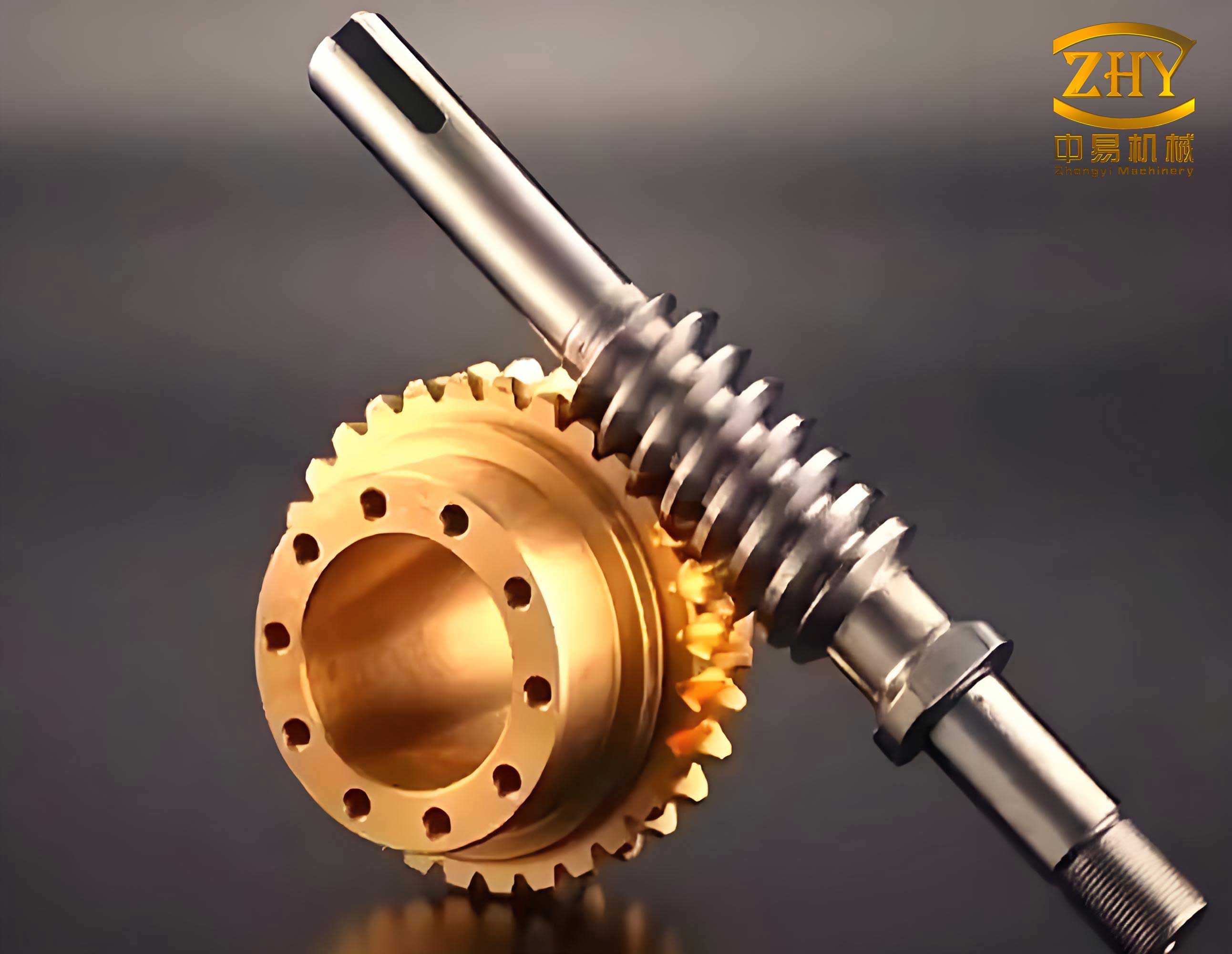
We begin by establishing the mathematical framework for high-order modified screw gear drives. The screw gear pair consists of a screw (worm) and a gear (worm wheel), where the screw tooth surface is generated by a straight-edge cutting tool. The modification is achieved by varying the process transmission ratio during the manufacturing of the screw, based on a high-order polynomial curve fitted from dimensionless modification data. This approach allows for a more accurate representation of wear patterns and improved meshing characteristics.
The core of our study lies in the derivation of the modification curve and its integration into the screw gear drive model. We collect modification data from empirical measurements and apply dimensionless processing to obtain universal modification curves. Using the least squares method, we fit the data with high-order polynomials, resulting in modification functions of the form:
$$ I_n(x) = \sum_{k=0}^{n} c_k x^k $$
where \( x \) is the angle coefficient, \( c_k \) are polynomial coefficients, and \( n \) represents the order of modification (e.g., \( n \geq 2 \)). For \( n=2 \), this reduces to parabolic modification, while \( n>2 \) corresponds to high-order modification. The coefficients for various orders are summarized in Table 1.
| Coefficient | 3rd Order Curve | 4th Order Curve | 5th Order Curve | 6th Order Curve | 7th Order Curve |
|---|---|---|---|---|---|
| \( c_0 \) | \( 9.9857 \times 10^{-2} \) | \( 1.0202 \times 10^{-1} \) | \( 1.0202 \times 10^{-1} \) | \( 9.6396 \times 10^{-2} \) | \( 9.640 \times 10^{-2} \) |
| \( c_1 \) | \( 5.0056 \times 10^{-1} \) | \( 5.0056 \times 10^{-1} \) | \( 5.2125 \times 10^{-1} \) | \( 5.2125 \times 10^{-1} \) | \( 5.1184 \times 10^{-1} \) |
| \( c_2 \) | \( 4.2790 \times 10^{-1} \) | \( 4.0739 \times 10^{-1} \) | \( 4.0739 \times 10^{-1} \) | \( 5.2004 \times 10^{-1} \) | \( 5.2004 \times 10^{-1} \) |
| \( c_3 \) | \( -4.5089 \times 10^{-2} \) | \( -4.5089 \times 10^{-2} \) | \( -1.3687 \times 10^{-1} \) | \( -1.3687 \times 10^{-1} \) | \( -5.5751 \times 10^{-2} \) |
| \( c_4 \) | 0 | \( -2.2659 \times 10^{-2} \) | \( 2.2659 \times 10^{-2} \) | \( -2.9935 \times 10^{-1} \) | \( -2.9935 \times 10^{-1} \) |
| \( c_5 \) | 0 | 0 | \( 7.8395 \times 10^{-2} \) | \( 7.8395 \times 10^{-2} \) | \( -9.2200 \times 10^{-2} \) |
| \( c_6 \) | 0 | 0 | 0 | \( 2.2474 \times 10^{-1} \) | \( 2.2474 \times 10^{-1} \) |
| \( c_7 \) | 0 | 0 | 0 | 0 | \( 1.0084 \times 10^{-1} \) |
The modification curve function is then expressed as:
$$ \Delta = \Delta_f I_n(x) = \Delta_f \sum_{k=0}^{n} c_k x^k $$
where \( \Delta_f \) is the modification amount at the entry point, calculated as \( \Delta_f = a(0.0003 + 0.000034 i_{12}) \), with \( a \) being the nominal center distance and \( i_{12} \) the gear ratio. This function directly influences the process transmission ratio \( i_{1d} \) during screw manufacturing. We derive the relationship between the modification curve and \( i_{1d} \) as:
$$ i_{1d} = \frac{i_{12}}{1 + \frac{\Delta_f}{r_2 \varphi_w} I_n'(x)} $$
where \( r_2 \) is the gear pitch radius, \( \varphi_w \) is the working half-angle, and \( I_n'(x) = \sum_{k=1}^{n} k c_k x^{k-1} \). This variable process transmission ratio is crucial for implementing high-order modification in screw gear drives.
Next, we develop the meshing theory for high-order modified screw gear drives. The screw tooth surface is generated by a straight-edge tool, and its equation in the screw coordinate system \( \sigma_1 \) is derived using rotation matrices. We represent the tool edge equation as:
$$ (\vec{r}_d)_d = -u \vec{i}_d + r_b \vec{j}_d $$
where \( u \) is the tool parameter and \( r_b \) is the base radius. Through coordinate transformations, the screw surface equation becomes:
$$ (\vec{r}_1)_1 = \vec{\rho}(\varphi) + u \vec{t}(\varphi) $$
This confirms that the screw tooth surface is a non-developable ruled surface, which aligns with the forming principle of screw gear drives. We then compute the fundamental quantities of the surface. The first fundamental form coefficients are:
$$ E = 1, \quad F = \frac{r_b}{i_{1d}}, \quad G = \frac{(x_{od} + a)^2 + (u^2 + r_b^2)}{i_{1d}^2} $$
where \( x_{od} = -u \cos \varphi_d – r_b \sin \varphi_d \), and \( \varphi_d \) is the tool rotation angle. The unit normal vector is:
$$ (\vec{n}_1)_1 = \frac{1}{D} \mathbf{R}[\vec{k}_1, -\varphi] \mathbf{R}\left[\vec{i}_{o1}, \frac{\pi}{2}\right] \mathbf{R}[\vec{k}_{od}, \varphi_d] \left[ (a + x_{od}) \vec{j}_d + \frac{u}{i_{1d}} \vec{k}_d \right] $$
with \( D = \sqrt{ \left( \frac{u}{i_{1d}} \right)^2 + (a + x_{od})^2 } \). The second fundamental form coefficients are:
$$ L = 0, \quad M = \frac{r_b \sin \varphi_d – a}{i_{1d} D}, \quad N = \frac{a + x_{od}}{D} \left[ (a + x_{od}) \sin \varphi_d – \left( u \frac{d^2\varphi_d}{d\varphi^2} – \frac{r_b}{i_{1d}^2} \right) \right] – \frac{2u y_{od}}{i_{1d}^2 D} $$
where \( y_{od} = -u \sin \varphi_d + r_b \cos \varphi_d \). From these, we determine the normal curvature \( k_\xi \), geodesic torsion \( \tau_\xi \), and mean curvature \( H \) along the tool direction:
$$ k_\xi = 0, \quad \tau_\xi = \frac{M}{D}, \quad H = \frac{N – 2FM}{2D^2} $$
These curvature parameters are essential for analyzing the meshing behavior of the screw gear pair.
We then derive the meshing function for the screw gear drive. The relative velocity between the screw and gear is computed, and the meshing function \( \Phi(u, \varphi, \varphi_1) \) is established as:
$$ \Phi(u, \varphi, \varphi_1) = (\vec{n}^*_1)_{o1} \cdot (\vec{V}_{12})_{o1} = \frac{1}{i_{12} D} \left[ A \sin(\varphi_1 – \varphi) + B \cos(\varphi_1 – \varphi) + C \right] $$
where \( A = \frac{u y_{od}}{i_{1d}} \), \( B = (x_{od} + a)(u – a \cos \varphi_d) \), and \( C = (x_{od} + a) \left( a \cos \varphi_d – \frac{i_{12}}{i_{1d}} u \right) \). The condition \( \Phi = 0 \) defines the contact points on the gear tooth surface. The gear surface equation in coordinate system \( \sigma_2 \) is:
$$ (\vec{r}_2)_2 = \mathbf{R}\left[\vec{k}_2, -\frac{\varphi_1}{i_{12}}\right] \left\{ \mathbf{R}\left[\vec{i}_{o2}, -\frac{\pi}{2}\right] (\vec{r}^*_1)_{o1} – a \vec{i}_{o2} \right\} = x_2 \vec{i}_2 + y_2 \vec{j}_2 + z_2 \vec{k}_2 $$
with \( x_2 = [(x_{od} + a) \cos(\varphi_1 – \varphi) – a] \cos\left(\frac{\varphi_1}{i_{12}}\right) + y_{od} \sin\left(\frac{\varphi_1}{i_{12}}\right) \), \( y_2 = [a – (x_{od} + a) \cos(\varphi_1 – \varphi)] \sin\left(\frac{\varphi_1}{i_{12}}\right) + y_{od} \cos\left(\frac{\varphi_1}{i_{12}}\right) \), and \( z_2 = -(x_{od} + a) \sin(\varphi_1 – \varphi) \).
Further, we compute the meshing limit function \( \Phi_{\varphi_1} \) and the curvature interference boundary function \( \Psi \):
$$ \Phi_{\varphi_1} = \frac{\partial \Phi}{\partial \varphi_1} = \frac{1}{i_{12} D} \left[ A \cos(\varphi_1 – \varphi) – B \sin(\varphi_1 – \varphi) \right] $$
$$ \Psi = N_\xi (\vec{V}_{12})_{o1} \cdot (\vec{\alpha}_\xi)_{o1} + N_\eta (\vec{V}_{12})_{o1} \cdot (\vec{\alpha}_\eta)_{o1} + \Phi_{\varphi_1} $$
where \( N_\xi \) and \( N_\eta \) are components of the normal vector to the instantaneous contact line. The induced normal curvature \( k_N^{(12)} \) and the sliding angle \( \theta_{vt} \) are given by:
$$ k_N^{(12)} = \frac{N_\xi^2 + N_\eta^2}{\Psi}, \quad \theta_{vt} = \arcsin\left( \frac{|\Psi – \Phi_{\varphi_1}|}{|(\vec{V}_{12})_{o1}| \sqrt{N_\xi^2 + N_\eta^2}} \right) $$
These parameters evaluate the local meshing quality of the screw gear drive, including contact stress and lubrication conditions.
To validate our theoretical model, we conduct numerical examples for screw gear drives with different modification orders. The basic parameters are: screw threads \( Z_1 = 2 \), center distance \( a = 280 \, \text{mm} \), gear ratio \( i_{12} = 25 \). Other derived parameters are listed in Table 2.
| Parameter | Calculation Method | Value |
|---|---|---|
| Screw pitch diameter (mm) | \( d_1 \approx 0.681 a^{0.875} \) | 94 |
| Gear pitch diameter (mm) | \( d_2 = 2a – d_1 \) | 466 |
| Gear face width (mm) | \( b_2 = 0.25a \) | 70 |
| Base diameter (mm) | \( d_b \approx 0.625a \) | 175 |
| Pressure angle (°) | \( \alpha = \arcsin\left( \frac{d_b}{d_2} \right) \) | 22.0589 |
| Gear teeth number | \( Z_2 = i_{12} Z_1 \) | 50 |
| Transverse module (mm) | \( m_t = \frac{d_2}{Z_2} \) | 9.3200 |
| Screw wrap angle (°) | \( \varphi_w = \frac{\pi}{Z_2} (Z_k – 0.5) \) | 16.3809 |
| Screw working length (mm) | \( L_w = d_2 \sin(\varphi_w) \) | 131.4151 |
| Screw addendum diameter (mm) | \( d_{a1} = d_1 + 1.5m_t \) | 107.98 |
| Gear addendum diameter (mm) | \( d_{a2} = d_2 + 1.5m_t \) | 479.98 |
| Entry point modification (mm) | \( \Delta_f = a(0.0003 + 0.000034 i_{12}) \) | 0.3239 |
We analyze the meshing characteristics for original (unmodified) and high-order modified screw gear drives. For the original screw gear drive with \( i_{1d} = i_{12} \), the conjugate region on the gear tooth surface degenerates into a constant contact line, leading to limited load capacity. In contrast, high-order modification eliminates this constant contact line and expands the conjugate region. For example, with third-order modification, the conjugate region is divided into two sub-regions: \( \Sigma_A \) and \( \Sigma_B \). The region \( \Sigma_A \) no longer degenerates, but it contains a curvature interference boundary where \( \Psi = 0 \). The region \( \Sigma_B \) expands to the screw exit, allowing full-length utilization of the screw. This improvement is consistent across higher-order modifications, such as fifth and seventh orders.
Table 3 summarizes the induced normal curvature \( k_N^{(12)} \) and sliding angle \( \theta_{vt} \) for the original screw gear drive at sample points. These points are selected at the intersections of instantaneous contact lines with the gear addendum, screw pitch circle, and screw addendum.
| Contact Line | Point a: \( k_N^{(12)} \, (\text{mm}^{-1}) \) | Point a: \( \theta_{vt} \, (°) \) | Point b: \( k_N^{(12)} \, (\text{mm}^{-1}) \) | Point b: \( \theta_{vt} \, (°) \) | Point c: \( k_N^{(12)} \, (\text{mm}^{-1}) \) | Point c: \( \theta_{vt} \, (°) \) |
|---|---|---|---|---|---|---|
| 1-5 (constant line) | 0 | – | 0 | – | 0 | – |
| 1′ | 0.0065 | 47.9606 | 0.0049 | 54.7752 | 0.0039 | 60.4146 |
| 2′ | 0.0052 | 53.1625 | 0.0039 | 59.7853 | 0.0032 | 64.9314 |
| 3′ | 0.0032 | 61.0311 | 0.0026 | 66.5065 | 0.0022 | 70.6119 |
| 4′ | 0.0013 | 73.5171 | 0.0012 | 76.2006 | 0.0011 | 78.1924 |
| 5′ | 0 | 0/0 | 0.0001 | 89.2260 | 0.0002 | 88.7754 |
For modified screw gear drives, the meshing quality improves. Table 4 shows results for third-order modification. The induced normal curvature in region \( \Sigma_A \) is relatively low, and the sliding angle is high, indicating favorable conditions for oil film formation. Similar trends are observed for fifth-order and seventh-order modifications, as detailed in Tables 5 and 6.
| Contact Line | Point a: \( k_N^{(12)} \, (\text{mm}^{-1}) \) | Point a: \( \theta_{vt} \, (°) \) | Point b: \( k_N^{(12)} \, (\text{mm}^{-1}) \) | Point b: \( \theta_{vt} \, (°) \) | Point c: \( k_N^{(12)} \, (\text{mm}^{-1}) \) | Point c: \( \theta_{vt} \, (°) \) |
|---|---|---|---|---|---|---|
| 1 | 0.1170 | 83.4593 | 0.0747 | 84.6715 | 0.0498 | 85.7864 |
| 1′ | 0.0076 | 50.9828 | 0.0066 | 56.0971 | 0.0059 | 61.4003 |
| 2′ | 0.0056 | 61.6673 | 0.0052 | 66.7319 | 0.0050 | 70.3258 |
| 3′ | 0.0026 | 83.9500 | 0.0027 | 83.0599 | 0.0028 | 82.6335 |
| 4′ | 0.0069 | 86.4867 | 0.0033 | 87.4160 | 0.0018 | 88.2022 |
| 5′ | 0.0155 | 83.1542 | 0.0086 | 82.4093 | 0.0047 | 80.6085 |
| Contact Line | Point a: \( k_N^{(12)} \, (\text{mm}^{-1}) \) | Point a: \( \theta_{vt} \, (°) \) | Point b: \( k_N^{(12)} \, (\text{mm}^{-1}) \) | Point b: \( \theta_{vt} \, (°) \) | Point c: \( k_N^{(12)} \, (\text{mm}^{-1}) \) | Point c: \( \theta_{vt} \, (°) \) |
|---|---|---|---|---|---|---|
| 1 | 0.0388 | 83.4708 | 0.0264 | 84.7314 | 0.0191 | 85.8765 |
| 1′ | 0.0066 | 51.5145 | 0.0056 | 56.3326 | 0.0048 | 61.5284 |
| 2′ | 0.0055 | 61.6975 | 0.0051 | 66.7762 | 0.0049 | 70.3822 |
| 3′ | 0.0027 | 83.8501 | 0.0028 | 82.9619 | 0.0029 | 82.5404 |
| 4′ | 0.0063 | 86.3912 | 0.0030 | 87.3020 | 0.0016 | 88.0843 |
| 5′ | 0.0339 | 83.4305 | 0.0212 | 82.8251 | 0.0140 | 81.3353 |
| Contact Line | Point a: \( k_N^{(12)} \, (\text{mm}^{-1}) \) | Point a: \( \theta_{vt} \, (°) \) | Point b: \( k_N^{(12)} \, (\text{mm}^{-1}) \) | Point b: \( \theta_{vt} \, (°) \) | Point c: \( k_N^{(12)} \, (\text{mm}^{-1}) \) | Point c: \( \theta_{vt} \, (°) \) |
|---|---|---|---|---|---|---|
| 1 | 0.0144 | 83.4178 | 0.0102 | 84.6668 | 0.0077 | 85.8115 |
| 1′ | 0.0047 | 55.2894 | 0.0039 | 59.4723 | 0.0031 | 64.3771 |
| 2′ | 0.0060 | 63.2244 | 0.0057 | 68.2945 | 0.0057 | 71.8984 |
| 3′ | 0.0025 | 83.8325 | 0.0026 | 83.3191 | 0.0026 | 83.0903 |
| 4′ | 0.0079 | 77.8907 | 0.0038 | 81.6272 | 0.0020 | 84.0717 |
| 5′ | 0.0092 | 78.7230 | 0.0049 | 70.9674 | 0.0025 | 73.1195 |
We also analyze the total fitting errors for different modification curves, as shown in Table 7. Increasing the polynomial order slightly reduces the error, but the improvement is marginal beyond a certain point.
| Curve Order | Total Error \( \sum_{i=1}^{35} [I_i – I(x^{(i)})]^2 \) |
|---|---|
| 2 | \( 6.9852 \times 10^{-2} \) |
| 3 | \( 5.4385 \times 10^{-2} \) |
| 4 | \( 5.3239 \times 10^{-2} \) |
| 5 | \( 4.9359 \times 10^{-2} \) |
| 6 | \( 3.9980 \times 10^{-2} \) |
| 7 | \( 3.9457 \times 10^{-2} \) |
Our numerical examples demonstrate that high-order modification effectively eliminates constant contact lines in screw gear drives, expands the conjugate region, and enables full-length utilization of the screw. This enhances the load capacity and durability of the screw gear pair. However, we note that curvature interference boundaries persist in the modified screw gear drives, particularly in region \( \Sigma_A \), which may lead to undercutting if not managed properly. For seventh-order modification, the interference boundary can be partially removed by trimming the gear tooth surface, but this requires careful design.
In conclusion, we have established a comprehensive mathematical model for high-order modified screw gear drives. Our derivations cover the modification curve fitting, process transmission ratio calculation, tooth surface geometry, and meshing analysis. The results show that high-order modification significantly improves the meshing performance of screw gear drives by increasing the contact area and optimizing curvature parameters. However, the presence of curvature interference boundaries suggests that high-order modification should be combined with other techniques, such as profile adjustments or hybrid modifications, to achieve optimal results. Future work could explore real-time adaptive modification strategies for screw gear drives in dynamic operating conditions.