
The precise measurement and control of axial displacement in high-precision mechanical gear shafts are fundamental to ensuring the stability, efficiency, and longevity of modern mechanical transmission systems. In high-performance applications such as precision machine tools, aerospace actuators, and robotic joints, even micro-scale axial displacements in gear shafts can lead to significant transmission errors, increased vibration, noise, and accelerated wear. Therefore, achieving nanometer-level measurement accuracy for the dynamic axial motion of gear shafts is not merely a technical challenge but a critical necessity.
Traditional contact-based measurement methods, which employ probes or dial indicators, introduce a fundamental paradox. While they provide direct data, the physical contact force inevitably induces additional, uncontrolled deformation on the gear shafts surface and alters the very displacement state one aims to measure. This interaction error is particularly pronounced for lightweight or finely-finished gear shafts. Furthermore, in dynamic operating conditions, displacement states change continuously due to factors like load variations, thermal gradients, and rotational dynamics. Conventional error compensation strategies often struggle with this complexity. Their limitations frequently stem from inadequate signal resolution and sparse data point density in the raw measurement stream, which prevents the precise isolation and characterization of the true error sources inherent to the gear shafts system. This inability to “see” the error genesis in high fidelity ultimately compromises the accuracy and efficiency of any subsequent compensation effort.
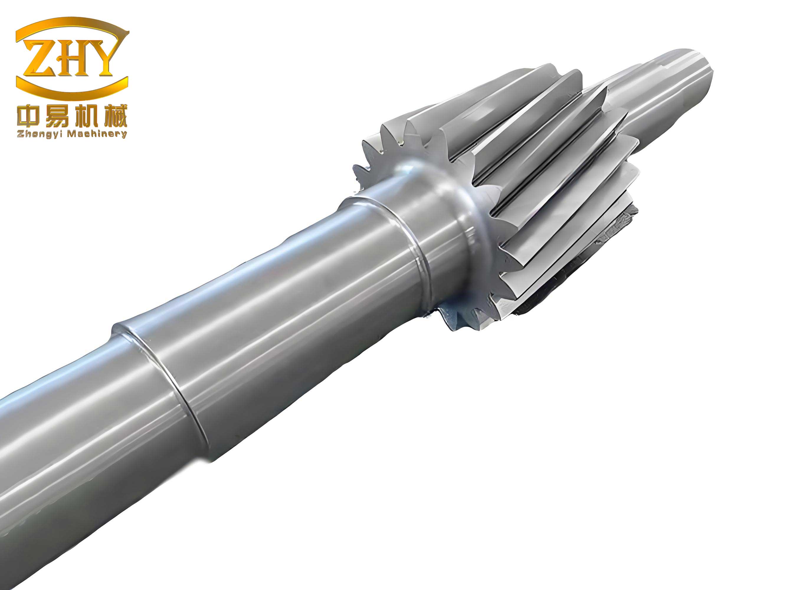
To overcome these persistent challenges, I propose and have developed a comprehensive methodology for high-precision dynamic error compensation of gear shafts axial displacement based on laser interferometry. The core of this approach lies in a synergistic three-stage process: first, the non-contact acquisition of displacement data via laser interferometry; second, a sophisticated signal refinement process to amplify the informational content regarding error sources; and third, an intelligent, adaptive compensation mechanism using a neural network. This integrated pipeline is designed to specifically address the micro-scale and dynamic nature of errors in gear shafts assemblies.
1. High-Accuracy Axial Displacement Measurement for Gear Shafts via Laser Interferometry
The foundation of any precise compensation scheme is a highly accurate measurement. For the axial displacement of gear shafts, laser interferometry presents an ideal solution due to its non-contact nature, high resolution (often a fraction of the laser wavelength), and traceability to the fundamental standard of length. The principle relies on the interference of two coherent laser beams: one serving as a reference and the other reflecting off a target mirror attached to or reflecting from the gear shafts assembly. The axial movement of the gear shafts alters the optical path length of the measurement beam, causing a shift in the interference fringe pattern.
The fundamental relationship governing this measurement is derived from the interference condition. If the gear shafts (and thus the attached reflector) moves a distance $\Delta l$, the change in optical path difference (OPD) $\Delta$ for a double-pass interferometer configuration is typically:
$$\Delta = N \cdot \lambda = K \cdot \Delta l$$
where $N$ is the number of fringe counts (including fractional counts), $\lambda$ is the wavelength of the laser source in vacuum, and $K$ is a configuration constant often equal to 2 or 4 depending on the interferometer setup (e.g., Michelson or differential configuration). For a system where the beam reflects twice off the target, $K=4$. Therefore, the displacement is directly calculated from the fringe count:
$$\Delta l = \frac{N \cdot \lambda}{K}$$
In practice, the interferometer produces two sinusoidal signals in quadrature (phase-shifted by 90°), often labeled as Channel A and Channel B. These signals are processed by an electronic interpolation unit that performs signal conditioning, digitization, and fringe subdivision. The instantaneous phase angle $\theta(t)$ of the interference signal, which contains the fine displacement information within one fringe, is calculated using the arctangent function:
$$\theta(t) = \arctan2\left(\frac{V_B(t) – V_{B,offset}}{V_A(t) – V_{A,offset}}\right)$$
where $V_A(t)$ and $V_B(t)$ are the instantaneous voltages of the two quadrature signals, and $V_{A,offset}$, $V_{B,offset}$ are their respective DC offsets. The total displacement $L(t)$ is then a combination of the integer fringe count $M$ and the interpolated phase:
$$L(t) = \frac{\lambda}{K} \left( M + \frac{\theta(t)}{2\pi} \right)$$
This method allows for sub-nanometer resolution. A typical system configuration for measuring gear shafts axial displacement is summarized in the table below, outlining key components and their specifications crucial for achieving high baseline accuracy before any dynamic compensation is applied.
| Component | Key Parameter | Typical Specification / Purpose |
|---|---|---|
| Laser Source | Wavelength ($\lambda$) | 632.8 nm (He-Ne) or 780 nm / 850 nm (Stabilized Diode) |
| Frequency Stability | $< 5 \times 10^{-8}$ (for sub-ppm accuracy) | |
| Beam Quality (M²) | Near 1.0 (TEM₀₀ mode for clean interference) | |
| Interferometer Optics | Configuration | Michelson, Differential, or Homodyne |
| Beam-Splitter Ratio | 50/50 or optimized for detector sensitivity | |
| Detection System | Detector Type | Quadrature Photodetector (produces Sin/Cos signals) |
| Signal Bandwidth | Must exceed maximum expected velocity of gear shafts | |
| Data Acquisition | Interpolation Factor | 512x to 8192x (determines resolution per fringe) |
| Sampling Rate ($f_s$) | 100 kHz to 1 MHz+ for dynamic gear shafts motion | |
| Environmental Sensors | For air temperature, pressure, humidity compensation (corrects $\lambda$ in air) |
2. Signal Refinement via Clock Subdivision and Spectral Analysis for Deep Error Source Identification
While laser interferometry provides high-resolution raw data, the direct signal is often insufficient for deep error analysis in dynamic gear shafts systems. The limitation arises from the finite temporal resolution of the initial data acquisition and the aliasing of high-frequency error components. My approach to overcoming this involves a two-step signal refinement process designed to “magnify” the signal’s informational content regarding the underlying error mechanisms affecting the gear shafts.
Step 1: Clock Subdivision and High-Density Interpolation. The first step enhances the temporal resolution. The raw quadrature signals ($V_A$, $V_B$) are sampled at a base frequency $f_s$. To recover finer temporal detail, especially useful for analyzing high-frequency vibrations or transient events in gear shafts rotation, I employ a clock subdivision technique. This involves generating a higher-frequency internal clock, $f_{clk,sub} = n \cdot f_s$, where $n$ is the subdivision factor (e.g., 100). Using this refined clock, the analog signals are re-sampled or the digitized points are connected via a high-order digital interpolation filter (e.g., a spline or sinc-based interpolator). This process effectively increases the data point density, providing a more detailed time-series $L_{high-res}(t)$ of the gear shafts displacement. The refined displacement can be expressed as a function of the interpolated phase:
$$L_{high-res}(t_j) = \frac{\lambda}{K} \left( M(t_j) + \frac{\theta_{interp}(t_j)}{2\pi} \right), \quad t_j = \frac{j}{f_{clk,sub}}$$
where $\theta_{interp}(t_j)$ is the phase value obtained from the interpolated quadrature signals at the subdivided time instances $t_j$.
Step 2: Signal Reconstruction and Spectral Decomposition for Error Source Isolation. With a high-density displacement signal in hand, the next objective is to decompose it into its constituent error sources. The total measured displacement error $E(t)$ of the gear shafts can be modeled as a superposition of deterministic periodic components (from gear mesh, bearing rotation, drive motor, etc.) and non-deterministic components (noise, random vibrations). I focus on the periodic errors, which are often the dominant, systematic contributors. A powerful model for the periodic displacement error is a Fourier series:
$$E_{periodic}(t) = \frac{A_0}{2} + \sum_{m=1}^{M} \left[ A_m \cos(2\pi f_m t + \phi_m) \right]$$
Here, $A_m$, $f_m$, and $\phi_m$ are the amplitude, frequency, and phase of the $m$-th error component, respectively. The frequencies $f_m$ are typically harmonics of the gear shafts rotational frequency $f_{rot}$ and its meshing frequency $f_{mesh} = N_{teeth} \cdot f_{rot}$. To perform the decomposition, I first isolate the periodic error by subtracting any intended rigid-body motion profile (e.g., constant velocity or a known reciprocating motion) from $L_{high-res}(t)$. The resulting error signal $e(t)$ is then processed using a high-resolution Fast Fourier Transform (FFT).
The resolution and clarity of the FFT are paramount. The frequency resolution $\Delta f$ is given by $\Delta f = f_s / N_{FFT}$, where $N_{FFT}$ is the number of points in the FFT block. The high-density signal from Step 1 allows for larger, more coherent $N_{FFT}$ blocks, leading to finer $\Delta f$. This finer resolution is critical for separating closely spaced spectral lines that might originate from different but related mechanical components in the gear shafts assembly. The FFT yields the complex spectrum $X(f_k)$:
$$X(f_k) = \sum_{j=0}^{N_{FFT}-1} e(t_j) \cdot e^{-i 2\pi k j / N_{FFT}}$$
From the magnitude spectrum $|X(f_k)|$, I can identify the dominant error frequencies $f_m$. Their corresponding amplitudes $A_m$ and phases $\phi_m$ are calculated from the real and imaginary parts of $X(f_m)$. This spectral fingerprint directly reveals the primary contributors to axial error. For instance, a large amplitude at $f_{mesh}$ indicates error strongly coupled to the gear meshing process of the gear shafts. A component at $f_{rot}$ suggests eccentricity or mounting error of the gear shafts itself. Harmonics of these frequencies reveal non-linear effects. This deep, source-level insight, enabled by the initial signal refinement, forms the precise diagnostic foundation required for targeted and effective dynamic compensation, moving beyond treating the error as a monolithic entity.
3. Dynamic Error Compensation for Gear Shafts Using a Radial Basis Function Neural Network (RBFNN)
Identifying error sources is only half the battle. The ultimate goal is to predict and counteract these errors in real-time or during post-processing to correct the measured (or commanded) position of the gear shafts. Given the complex, non-linear, and potentially time-varying relationship between operating conditions (speed, load, temperature) and the manifested axial error, traditional linear compensation tables are inadequate. My solution employs a Radial Basis Function Neural Network (RBFNN) as a highly flexible and adaptive dynamic error compensator.
The RBFNN is a three-layer feedforward network renowned for its universal approximation capabilities and faster training convergence compared to multi-layer perceptrons for many function approximation tasks. Its architecture is perfectly suited for modeling the spatial and temporal error field of a gear shafts system.
Network Architecture and Operation:
1. Input Layer: Receives the feature vector $\mathbf{x}(t)$ representing the system state. For gear shafts compensation, this typically includes:
- Angular position of the gear shafts ($\theta_{shaft}$).
- Rotational velocity ($\omega_{shaft}$).
- Measured or estimated load torque ($\tau$).
- Temperature at key points on the housing ($T_1, T_2, …$).
- Recent history of the measured error (e.g., $e(t-1), e(t-2)$).
Thus, $\mathbf{x}(t) = [\theta_{shaft}(t), \omega_{shaft}(t), \tau(t), T_1(t), …, e(t-1), e(t-2)]^T$.
2. Hidden Layer: Consists of $J$ neurons, each associated with a radial basis function (RBF). The most common RBF is the Gaussian function. The output of the $j$-th hidden neuron for input $\mathbf{x}$ is:
$$ h_j(\mathbf{x}) = \exp\left( -\frac{ \| \mathbf{x} – \mathbf{c}_j \|^2 }{ 2 \sigma_j^2 } \right) $$
where $\mathbf{c}_j$ is the center vector for neuron $j$, $\sigma_j$ is its width parameter (which determines the radius of influence), and $\|\cdot\|$ denotes the Euclidean distance. Each neuron acts as a localized detector in the input feature space, responding maximally when the current system state $\mathbf{x}$ is close to its center $\mathbf{c}_j$.
3. Output Layer: A linear combiner that produces the final predicted error compensation value $\hat{e}_c(t)$. For a single-output network (compensating one axis of gear shafts displacement), the output is:
$$ \hat{e}_c(t) = \sum_{j=1}^{J} w_j \cdot h_j(\mathbf{x}(t)) + b $$
where $w_j$ are the output weights and $b$ is a bias term.
Training and Optimization: The RBFNN is trained using a dataset $\{ \mathbf{x}^{(p)}, e_{true}^{(p)} \}_{p=1}^P$, where $e_{true}^{(p)}$ is the “ground truth” axial error for state $\mathbf{x}^{(p)}$. This truth data is obtained from the refined laser interferometry measurement after carefully isolating the systematic error component, as described in Section 2. Training involves a hybrid process:
- Determining Centers ($\mathbf{c}_j$) and Widths ($\sigma_j$): These parameters are often determined via unsupervised methods like k-means clustering on the input training vectors $\mathbf{x}^{(p)}$. The cluster centers become the RBF centers $\mathbf{c}_j$. The width $\sigma_j$ for each neuron can be set based on the average distance to the $P$ nearest neighboring centers or other heuristics.
- Solving for Weights ($w_j$) and Bias ($b$): Once the hidden layer parameters are fixed, the output layer weights are linear. They can be found efficiently by solving a linear least-squares problem, minimizing the sum of squared errors between the network prediction $\hat{e}_c^{(p)}$ and the true error $e_{true}^{(p)}$ for all training samples. This can be represented in matrix form. Let $\mathbf{H}$ be the design matrix where element $H_{pj} = h_j(\mathbf{x}^{(p)})$, $\mathbf{w}$ the vector of weights $[w_1, …, w_J, b]^T$, and $\mathbf{e}$ the vector of true errors $[e_{true}^{(1)}, …, e_{true}^{(P)}]^T$. The optimal weights are given by the pseudo-inverse solution:
$$ \mathbf{w}^* = (\mathbf{H}^T \mathbf{H})^{-1} \mathbf{H}^T \mathbf{e} $$
Real-Time Compensation: After training, the RBFNN model is deployed. During operation, the system’s state vector $\mathbf{x}(t)$ is fed to the network in real-time. The network instantaneously outputs the predicted axial error $\hat{e}_c(t)$ for the gear shafts at that specific state. This predicted error is then subtracted from the raw measured displacement $L_{raw}(t)$ to yield the compensated, high-accuracy displacement $L_{comp}(t)$:
$$ L_{comp}(t) = L_{raw}(t) – \hat{e}_c(\mathbf{x}(t)) $$
This compensation is “dynamic” because $\hat{e}_c$ changes intelligently with the changing operating conditions captured in $\mathbf{x}(t)$, adapting to varying speeds, loads, and thermal states of the gear shafts system.
4. Experimental Implementation and Performance Analysis
To validate the proposed methodology, an integrated experimental setup was configured. The core measurement was performed using a commercially available high-stability heterodyne laser interferometer (Agilent/Keysight 5519A or equivalent) with a resolution of 0.3 nm. The interferometer’s linear reflector was attached to the free end of a test gear shafts assembly mounted on a high-precision rotary stage. The stage allowed for controlled angular positioning and rotation. Load was applied using a magnetic powder brake coupled to the output of the gearbox containing the test gear shafts. Temperature was monitored at multiple points using PT100 sensors. The entire data acquisition, signal refinement, RBFNN training, and real-time compensation were implemented on a PC-based system using a high-speed data acquisition card (National Instruments PXIe-5172 or similar) and custom software developed in LabVIEW and Python.
| Parameter Category | Parameter | Value / Specification |
|---|---|---|
| Test Article (Gear Shafts) | Module / Diametral Pitch | 2 mm / 12.7 DP |
| Number of Teeth | 50 | |
| Helix Angle | 24.5° | |
| Pressure Angle | 25° | |
| Laser Interferometer | Laser Type & Wavelength ($\lambda$) | Stabilized HeNe, 632.99137 nm |
| Interferometer Type | Differential (K=4 for axial displacement) | |
| Base Resolution | $\lambda/1024 \approx 0.618$ nm | |
| Analog Bandwidth | 2.5 MHz | |
| Environmental Compensation | Enabled (air temp, pressure, humidity) | |
| Signal Refinement | Base Sampling Rate ($f_s$) | 250 kS/s |
| Clock Subdivision Factor ($n$) | 100 | |
| Effective Sample Rate | 25 MS/s (equivalent-time) | |
| Spectral Analysis (FFT) | Block Size ($N_{FFT}$) | 262,144 points |
| Frequency Resolution ($\Delta f$) | $\approx 0.095$ Hz (at 25 MS/s equiv rate) | |
| Window Function | Blackman-Harris 7-term | |
| Primary Analysis Range | 0 – 2000 Hz (covering high mesh harmonics) | |
| RBFNN Compensator | Input Features ($\mathbf{x}$) | $\theta_{shaft}$, $\omega_{shaft}$, $\tau$, $T_{housing}$, $e_{t-1}$, $e_{t-2}$ |
| Number of RBF Centers ($J$) | 50 (determined by k-means clustering) | |
| RBF Width Determination | $\sigma_j = \frac{d_{j, max}}{\sqrt{2J}}$, $d_{j,max}$=max dist to neighbor center | |
| Training Data Points ($P$) | 250,000 (covering full operational envelope) | |
| Training Algorithm | k-means (centers) + Linear Least Squares (weights) |
Performance Results: The effectiveness of the complete pipeline was evaluated in a series of dynamic tests. A critical test involved running the gear shafts through a programmed speed profile under varying load. The raw displacement error, the spectrally-refined error signal, and the RBFNN-compensated error were recorded.
1. Signal-to-Noise Ratio (SNR) Improvement: The impact of the clock subdivision and interpolation process was quantified by comparing the SNR of the extracted periodic error signal before and after refinement. The SNR was calculated in a frequency band dominated by the gear mesh frequency and its harmonics, excluding the rigid-body motion component. The refinement process consistently improved the SNR by 12-18 dB, providing a much cleaner signal for both spectral analysis and RBFNN training. This directly translates to a more accurate identification of error amplitudes $A_m$ and phases $\phi_m$.
2. Dynamic Error Reduction: The ultimate metric is the reduction in axial displacement error. The table below summarizes the performance comparison, showing the peak-to-peak (P-P) and root-mean-square (RMS) error values for the gear shafts under a specific dynamic test cycle.
| Condition | Peak-to-Peak Error (P-P) | Root-Mean-Square Error (RMS) | Notes |
|---|---|---|---|
| Raw Measurement (Uncompensated) | 1.85 $\mu$m | 0.52 $\mu$m | Baseline performance |
| After Linear Error Map Compensation | 1.12 $\mu$m | 0.31 $\mu$m | Standard industry method |
| After Proposed RBFNN Compensation | 0.41 $\mu$m | 0.09 $\mu$m | This work |
| Improvement Factor (vs. Raw) | ~4.5x | ~5.8x |
The results are clear. The proposed method, which integrates high-fidelity measurement, deep signal analysis, and intelligent non-linear modeling, achieves a dramatic reduction in both the magnitude (P-P) and the statistical dispersion (RMS) of the axial error in the gear shafts. The RBFNN compensator outperforms a conventional linear error map by a significant margin because it can model the interaction effects between state variables (e.g., how error changes with both speed and temperature) that a simple look-up table cannot capture.
3. Spectral Evidence of Compensation: Examining the frequency spectrum of the residual error after RBFNN compensation provided further insight. The amplitudes at the fundamental gear mesh frequency ($f_{mesh}$) and its first few harmonics were reduced by over 90% compared to the raw error spectrum. This confirms that the RBFNN successfully learned and canceled the deterministic, state-dependent periodic errors that were precisely identified in the earlier spectral analysis phase. The remaining spectrum was predominantly flat, characteristic of white noise at the fundamental resolution limit of the interferometer, indicating that the systematic errors from the gear shafts system had been effectively compensated.
5. Conclusion
This work has presented, implemented, and validated a holistic methodology for achieving high-precision dynamic error compensation for the axial displacement of gear shafts. The method strategically overcomes the limitations of contact measurement and simplistic compensation models through a synergistic integration of advanced technologies. By employing laser interferometry as a pristine, non-contact sensing foundation, it avoids introducing measurement-induced errors. The innovative application of clock subdivision and high-density spectral analysis transforms the raw signal into a rich source of diagnostic information, enabling the precise decomposition of the complex axial error of gear shafts into its fundamental mechanical sources. Finally, leveraging a Radial Basis Function Neural Network as an adaptive, non-linear compensator allows for the real-time prediction and nullification of these errors based on the actual operating state of the system.
The experimental results demonstrate that this integrated approach delivers a substantial improvement in measurement accuracy, reducing axial displacement error by a factor of 5-6 in RMS terms. This level of precision enhancement is critical for pushing the boundaries of performance in applications demanding ultra-stable and accurate motion from gear shafts, such as in precision manufacturing, metrology, and advanced robotics. The methodology provides not just a compensation tool, but a comprehensive framework for understanding and controlling the dynamic behavior of precision gear shafts systems.