
The continuous evolution of mechanical systems demands ever-higher standards for power transmission components, with cylindrical gears remaining a cornerstone. Among various manufacturing techniques, gear hobbing stands out due to its efficiency and versatility in generating involute profiles. However, the physical process of gear hobbing involves complex interactions between the cutting tool and the workpiece, making it challenging to predict final gear quality and optimize process parameters solely through trial-and-error. This is where high-fidelity computer simulation becomes an indispensable tool. It allows for the virtual exploration of the gear hobbing process, enabling the prediction of tooth surface geometry, the analysis of potential errors, and the optimization of cutting conditions before any metal is cut. This article details a robust methodology for simulating high-precision gear hobbing based on the CATIA V5 platform, coupled with a rigorous mathematical framework for validating the accuracy of the resulting virtual gear model.
Fundamental Principles of Gear Hobbing
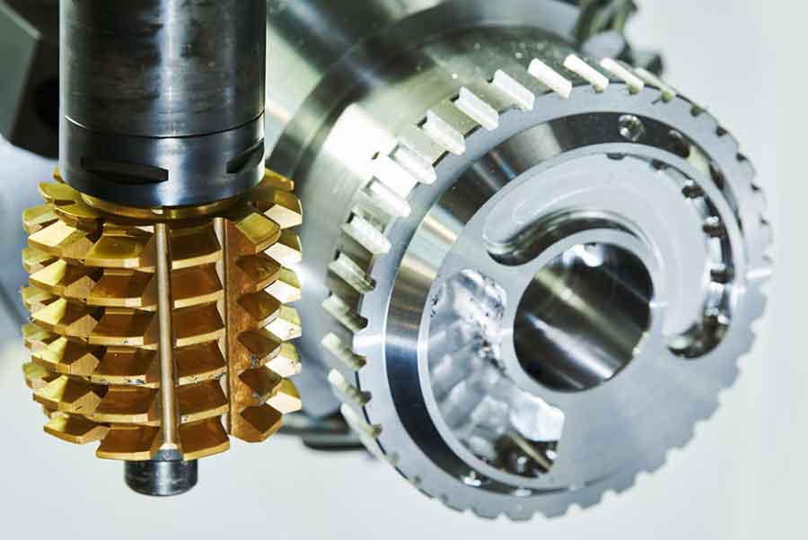
At its core, gear hobbing is a continuous form-cutting process based on the principle of generating milling. The hob, which can be conceptualized as a worm gear with gashes to form cutting edges, and the gear blank maintain a strict kinematic relationship mimicking the meshing of a worm and worm wheel. The relative motions between the hob and the blank are decomposed into three primary components for spur gears, with an additional motion required for helical gears.
1. Primary Cutting Motion (C1): This is the rotation of the hob around its own axis at a constant angular velocity \(\omega_h\).
2. Generating Motion (C2 & C3): To maintain the correct meshing condition, the rotation of the hob must be synchronized with the rotation of the gear blank. This relationship is defined by the gear ratio:
$$ \frac{\omega_w}{\omega_h} = \frac{N_h}{Z} $$
where \(\omega_w\) is the angular velocity of the workpiece, \(N_h\) is the number of starts on the hob (usually 1 for standard hobs), and \(Z\) is the number of teeth to be cut on the gear. This combined rotation simulates the rolling action of a theoretical rack against the gear blank.
3. Feed Motion (F): To cut the gear teeth along the entire face width, the hob or the blank must move radially (for plunge hobbing) or axially (for traverse hobbing). In the common traverse gear hobbing method, the hob travels parallel to the axis of the gear blank. This axial feed rate, denoted as \(f_a\) (mm per revolution of the workpiece), determines the productivity and surface finish.
4. Differential Motion for Helical Gears (Cd): When cutting a helical gear, an additional rotary motion must be superimposed on the workpiece rotation. This differential motion ensures that the axial travel of the hob is synchronized with the required helix lead of the gear. The relationship is given by:
$$ \text{Additional rotation per axial feed} = \frac{f_a \cdot \tan(\beta)}{r_p} $$
where \(\beta\) is the helix angle and \(r_p\) is the pitch radius of the workpiece. This forces the cutting process to follow the helical path.
In the virtual domain, these motions are replicated by applying successive translational and rotational transformations to the digital models of the hob and the blank, followed by Boolean subtraction operations to simulate material removal.
High-Precision Simulation Methodology in CATIA
The proposed simulation method enhances precision and computational efficiency by strategically decomposing the gear hobbing process into two distinct phases. This approach minimizes redundant calculations and memory usage inherent in simulating every single hob tooth engagement across the full face width.
Phase 1: Extraction of the Preliminary Tooth Slot Model
The objective of this phase is to generate a single, representative tooth slot that encapsulates all geometric features imparted by the primary cutting and generating motions, excluding the effects of the axial feed.
Step 1: Model Preparation. A simplified, yet kinematically accurate, 3D model of the hob is created. For simulation purposes, features like chip flutes and complex rake faces can be simplified, focusing instead on the precise involute helicoid profile of the hob’s cutting threads. Key parameters of a sample hob model are listed below:
| Parameter | Value | Parameter | Value |
|---|---|---|---|
| Normal Module | 2 mm | Number of Starts | 1 |
| Outside Diameter | 80 mm | Axial Pitch | 6.283 mm |
| Pressure Angle | 20° | Helix Angle | 1.55° |
The gear blank is modeled as a simple cylinder with dimensions corresponding to the gear’s outer diameter and face width. The target helical gear specifications are:
| Parameter | Value | Parameter | Value |
|---|---|---|---|
| Number of Teeth (Z) | 20 | Helix Angle (β) | 20° (Right Hand) |
| Normal Module (m_n) | 2 mm | Face Width | 20 mm |
| Normal Pressure Angle (α_n) | 20° | Profile Shift Coefficient | 0 |
Step 2: Kinematic Simulation and Boolean Subtraction. The hob is positioned at the nominal depth of cut at the midpoint of the gear blank’s face width. A macro program is developed to automate the following sequence in a loop:
- Rotate the hob by a small angular increment \(\Delta\theta_h\). This increment is typically \(\Delta\theta_h = 2\pi / n\), where \(n\) is the number of discrete simulation steps per hob revolution, often chosen as a multiple of the virtual hob’s tooth count for completeness.
- Rotate the gear blank by a corresponding angle \(\Delta\theta_w = \Delta\theta_h \cdot (N_h / Z)\) to maintain the generating motion.
- Perform a Boolean subtraction (Cut) operation, removing the volume occupied by the hob from the gear blank.
This loop continues until the hob has theoretically completed several full rotations around the blank, ensuring a fully developed, precise tooth slot profile is enveloped at that specific axial cross-section. The resulting entity is the Preliminary Tooth Slot Model.
Phase 2: Axial Feed Simulation using the Preliminary Model
Instead of continuing with the complex hob model, the preliminary tooth slot model—which already contains the exact generating profile—is used as a cutting tool. This drastically reduces geometric complexity.
Step 3: Traverse and Differential Motion Simulation. Another macro controls this phase:
- Translate the preliminary tooth slot model axially along the gear blank by the axial feed increment \(f_a\).
- Simultaneously, apply the differential rotation to the tooth slot model (or, equivalently, to the blank) around the gear axis. The rotation angle \(\Delta\gamma\) for a feed increment \(f_a\) is: $$ \Delta\gamma = \frac{f_a \cdot \tan(\beta)}{r_p} $$
- Perform a Boolean subtraction of the translated and rotated preliminary model from the gear blank.
This process is repeated step-by-step until the entire face width is traversed. The final result is a single, high-precision tooth slot that accurately reflects the combined effects of all gear hobbing motions.
Step 4: Pattern Completion. The completed tooth slot is circumferentially patterned \(Z\) times (e.g., 20 times) around the gear axis. A final Boolean subtraction of this pattern from the original gear blank cylinder yields the complete, simulated helical gear.
Mathematical Framework for Accuracy Validation
Verifying the accuracy of the virtual gear is crucial. This is achieved by comparing the simulated tooth surface against a mathematically perfect theoretical surface.
Generation of the Reference Tooth Surface Point Cloud
The theoretical tooth surface of a helical gear is a complex 3D involute helicoid. A discrete point cloud representing this surface is generated for measurement. For any point on the transverse section, the coordinates of an involute are given by:
$$ x = r_b (\sin(\theta) – \theta\cos(\theta)) $$
$$ y = r_b (\cos(\theta) + \theta\sin(\theta)) $$
where:
- \(r_b\) is the base circle radius in the transverse plane, \(r_b = r_p \cos(\alpha_t)\).
- \(\alpha_t\) is the transverse pressure angle, \(\alpha_t = \arctan(\tan(\alpha_n) / \cos(\beta))\).
- \(\theta\) is the involute roll angle.
To account for the helical nature, this transverse involute point is transformed along the helix. A series of transverse planes are defined along the face width. For a point in plane \(j\) at axial position \(z_j\), an additional rotation \(\phi_j\) is applied to the involute coordinates:
$$ \phi_j = \frac{z_j \cdot \tan(\beta)}{r_p} $$
The 3D coordinates \((X_j, Y_j, Z_j)\) of the point cloud are thus:
$$ X_j = x \cos(\phi_j) – y \sin(\phi_j) $$
$$ Y_j = x \sin(\phi_j) + y \cos(\phi_j) $$
$$ Z_j = z_j $$
By varying \(\theta\) and \(z_j\) systematically, a dense cloud of points representing the ideal left and right flanks is created and imported into the CATIA environment containing the simulated gear.
Error Measurement and Analysis
The normal distance from each point in the theoretical cloud to the corresponding simulated tooth surface is measured using CATIA’s surface distance analysis tool. This yields a set of error values \(\delta_i\) for \(i = 1\) to \(N\) points. Key metrics are calculated:
- Maximum Error (\(\delta_{max}\)): $$ \delta_{max} = \max(|\delta_i|) $$
- Root Mean Square Error (\(\delta_{RMS}\)): $$ \delta_{RMS} = \sqrt{\frac{1}{N}\sum_{i=1}^{N} \delta_i^2} $$
The spatial distribution of \(\delta_i\) can be plotted to visualize error patterns, such as systematic deviations or periodic marks corresponding to the feed rate.
Simulation Results and Parametric Analysis
Applying the described methodology, multiple virtual gear hobbing simulations were run with varying key parameters: hob tooth count (\(N_t\)) and axial feed per revolution (\(f_a\)). The primary metric for comparison was the maximum normal error \(\delta_{max}\) on the tooth flank. The table below summarizes findings for a 12-tooth and a 24-tooth hob simulation.
| Hob Tooth Count (Nt) | Maximum Surface Error \(\delta_{max}\) (µm) for Feed \(f_a\) | |||
|---|---|---|---|---|
| 1 mm/rev | 2 mm/rev | 3 mm/rev | 4 mm/rev | |
| 12 | 1.58 | 4.71 | 9.50 | 20.36 |
| 24 | 0.97 | 4.69 | 9.05 | 20.22 |
Analysis of Results:
1. Effect of Axial Feed (\(f_a\)): The most significant factor influencing simulation accuracy is the axial feed. As \(f_a\) increases, \(\delta_{max}\) increases substantially. This is a direct digital analog to the physical process: a larger feed creates a more pronounced “step” or cusp height between successive tool positions. The relationship is nonlinear, with error escalating rapidly at higher feeds. The simulation accurately captures this fundamental trade-off between productivity (high feed) and surface finish (low feed) in real gear hobbing.
2. Effect of Hob Tooth Count (\(N_t\)): The number of teeth on the virtual hob influences the circumferential sampling of the generating motion. A higher tooth count (e.g., 24 vs. 12) provides a finer discretization of the hob’s rotation, leading to a smoother envelope and slightly lower error, particularly at smaller feed rates. This mirrors the practice of using finer-pitch hobs for precision finishing operations in actual gear hobbing. The effect becomes less pronounced at very high feeds where the axial feed error dominates.
3. Error Distribution Pattern: Plotting the error values across the tooth surface reveals a characteristic wavy pattern. The peaks of error are aligned along the paths corresponding to the axial feed increments—the virtual “feed marks.” The valleys lie between these paths. This pattern provides critical insight into how process parameters in gear hobbing translate directly into topographical features on the gear tooth, which can affect noise, vibration, and lubrication performance.
Conclusion and Implications
The developed framework establishes a high-precision digital twin for the gear hobbing process. By leveraging CATIA’s robust geometric kernel and automation capabilities through a two-phase simulation strategy, it successfully generates virtual gear models with sub-micron level geometric fidelity when using fine process parameters. The integrated mathematical validation method, based on a theoretical involute helicoid point cloud, provides a quantitative and spatially detailed assessment of tooth surface accuracy.
This virtual platform serves multiple critical functions in advanced gear manufacturing:
- Process Planning & Optimization: Engineers can virtually test the outcome of different combinations of hob design, feed rates, and speeds without consuming material or machine time, identifying the set that minimizes surface error or reduces cycle time.
- Root Cause Analysis: Deviations in the simulated gear from its ideal form can be traced back to specific kinematic parameters or model assumptions, aiding in troubleshooting real-world gear hobbing quality issues.
- Tool Path Verification: For CNC hobbing machines, the simulated kinematics can be used to verify the correctness of machine tool paths.
- Foundation for Advanced Analysis: The highly accurate 3D gear model serves as a perfect input for subsequent finite element analysis (FEA) for stress, thermal, or dynamic studies, ensuring those analyses start from a geometrically correct basis.
Furthermore, the core methodology—separating the generation of a precise profile from its axial propagation—is not limited to gear hobbing. It is readily adaptable to simulate other generating gear processes such as shaping and grinding, providing a unified approach for virtual gear manufacturing analysis and validation. This work bridges the gap between digital modeling and physical manufacturing, offering a powerful tool for achieving first-part-correct production in precision gear machining.