
In this study, I investigate the dynamic characteristics and modification optimization of a high-speed train helical gear pair under multiple operating conditions. The helical gear is one of the most important components in a train transmission system, and its dynamic behavior directly influences ride comfort, safety, reliability, and acoustic performance. Because high-speed trains operate under rapidly changing torque and speed conditions, a modification scheme optimized for only one nominal condition may not remain effective over the full service range. Therefore, I establish a multi-degree-of-freedom dynamic model, evaluate several representative working conditions, construct a data-driven prediction model, and apply a genetic algorithm to obtain a comprehensive modification strategy for the helical gear pair.
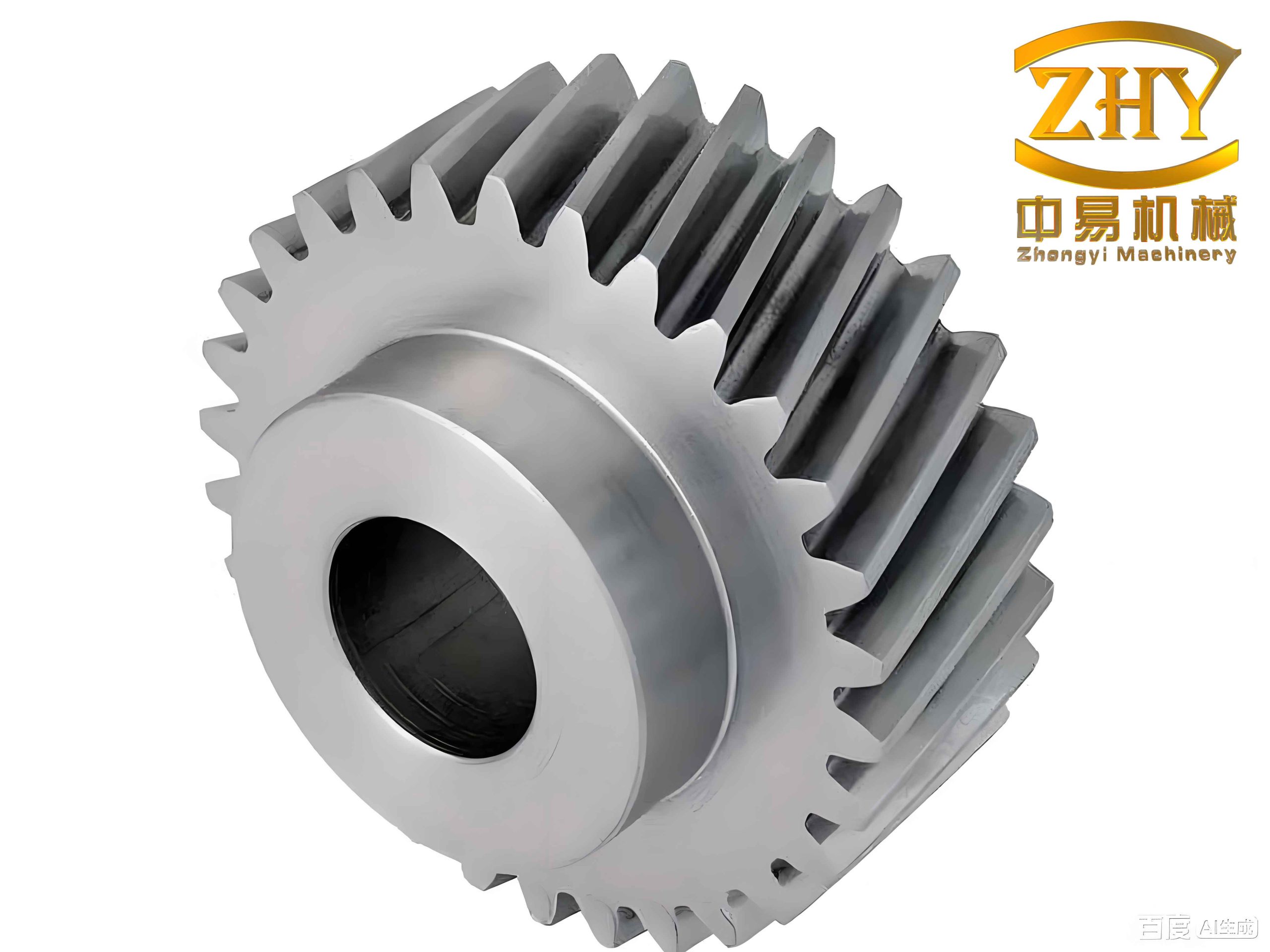
Motivation and Scope
I focus on a parallel-axis helical gear system because helical gears are widely used in high-speed train transmissions due to their smooth meshing, high load capacity, and lower noise compared with spur gears. Nevertheless, the helical gear pair still experiences time-varying mesh stiffness, friction, transmission error, and backlash nonlinearity. These effects produce vibration and impact, especially when the operating torque and rotational speed vary. Tooth profile modification and lead modification are effective methods for reducing the abrupt change in mesh stiffness and the peak-to-peak dynamic transmission error. My objective is to determine a set of modification parameters that performs well across nine main operating conditions rather than only at a single rated condition.
Dynamic Model of the Helical Gear Pair
I use the lumped-parameter method to represent the helical gear transmission. The model includes translational and torsional motions, and I consider the mesh stiffness, mesh damping, friction, static transmission error, and backlash. The generalized coordinate vector is written as
$$
\mathbf{q}=[x_1,x_2,y_1,y_2,\theta_1,\theta_2]^T
$$
where \(x_i\) and \(y_i\) are the translational displacements of the driving and driven helical gears, and \(\theta_i\) are their angular displacements. The global dynamic equation of the helical gear system is expressed as
$$
\mathbf{M}\ddot{\mathbf{q}}+\mathbf{C}\dot{\mathbf{q}}+\mathbf{K}\mathbf{q}=\mathbf{P}
$$
where \(\mathbf{M}\), \(\mathbf{C}\), and \(\mathbf{K}\) are the mass, damping, and stiffness matrices, respectively, and \(\mathbf{P}\) is the excitation vector. The mass matrix contains the gear masses and rotary inertias. The stiffness and damping matrices include the bearing support terms and the mesh coupling terms. Because the mesh stiffness of a helical gear changes periodically with the contact position, the stiffness matrix is time dependent.
The dynamic mesh force along the line of action is written as
$$
F_m(t)=k_m(t)f(\delta)+c_m\dot{\delta}
$$
where \(k_m(t)\) is the time-varying mesh stiffness, \(c_m\) is the mesh damping, and \(f(\delta)\) is the backlash function. The relative mesh deformation is
$$
\delta(t)=x_1-x_2+R_{b1}\theta_1-R_{b2}\theta_2-e(t)
$$
in which \(R_{b1}\) and \(R_{b2}\) are the base circle radii of the driving and driven helical gears, and \(e(t)\) is the static transmission error. The backlash nonlinearity is described by
$$
f(\delta)=
\begin{cases}
\delta-b_n, & \delta \gt b_n \\
0, & -b_n \le \delta \le b_n \\
\delta+b_n, & \delta \lt -b_n
\end{cases}
$$
where \(b_n\) is the half backlash. This piecewise function allows the helical gear teeth to remain in contact, lose contact, or re-enter contact. Such behavior is important because the dynamic transmission error of a helical gear pair can be strongly affected by backlash, especially under light load or reversing conditions.
The dynamic transmission error of the helical gear pair is defined as
$$
TE(t)=x_1-x_2+R_{b1}\theta_1-R_{b2}\theta_2-e(t)
$$
and the peak-to-peak value of \(TE(t)\) is used as a key indicator of vibration and meshing quality. A smaller peak-to-peak dynamic transmission error generally indicates smoother motion and lower excitation of the gearbox housing.
External Excitation and Operating Conditions
I select nine main operating conditions for the high-speed train helical gear pair. These conditions cover low-speed startup, intermediate-speed cruising, and high-speed operation. The motor speed, motor torque, vehicle speed, and power are listed in Table 1. The torque generally decreases as speed increases, while the power rises and then levels off. The nine conditions allow me to evaluate the helical gear dynamic response over a broad range instead of relying on a single nominal point.
| Condition | Motor speed (rpm) | Motor torque (N·m) | Vehicle speed (km/h) | Power (kW) |
|---|---|---|---|---|
| 1 | 80 | 9000 | 5 | 75.39 |
| 2 | 125 | 8830 | 8 | 115.57 |
| 3 | 230 | 9890 | 12 | 238.18 |
| 4 | 1500 | 7140 | 80 | 1121.46 |
| 5 | 1900 | 6750 | 100 | 1342.93 |
| 6 | 2250 | 6020 | 120 | 1418.32 |
| 7 | 3500 | 3960 | 180 | 1451.30 |
| 8 | 3800 | 3590 | 200 | 1428.48 |
| 9 | 4150 | 3220 | 220 | 1399.26 |
Internal Excitation of the Helical Gear Pair
The internal excitation of the helical gear pair mainly includes time-varying mesh stiffness, time-varying friction, mesh damping, and static transmission error. I calculate the time-varying friction coefficient using a thermal elastohydrodynamic lubrication model. The friction coefficient depends on the sliding speed, entrainment speed, contact pressure, surface roughness, and lubricant viscosity. I use the following form:
$$
\mu=b_1\Phi(S,R_h,\nu_0,V_s)S^{b_2}R_h^{b_3}V_e^{b_6}\nu_0^{b_7}V_s^{b_8}
$$
with
$$
\Phi(S,R_h,\nu_0,V_s)=1+b_4\frac{S}{R_h}\frac{V_e}{\nu_0}+b_5e^{-S/R_h}\frac{V_e}{\nu_0}+b_9S
$$
The empirical coefficients used in my calculation are given in Table 2. The friction coefficient is not constant during a mesh cycle. It tends to decrease near the pitch point because the relative sliding velocity approaches zero there, and it increases away from the pitch point where sliding becomes more pronounced.
| Coefficient | Value |
|---|---|
| \(b_1\) | -8.92 |
| \(b_2\) | 1.03 |
| \(b_3\) | 1.04 |
| \(b_4\) | -0.35 |
| \(b_5\) | 2.81 |
| \(b_6\) | -0.10 |
| \(b_7\) | 0.75 |
| \(b_8\) | -0.39 |
| \(b_9\) | 0.62 |
For mesh stiffness, I adopt an improved Ishikawa formula. The helical gear tooth is simplified as a combination of rectangular and trapezoidal sections. The total deformation along the line of action is the sum of the bending deformation, shear deformation, foundation deformation, and contact deformation. The mesh stiffness is then obtained from
$$
k=\frac{F_n}{b\delta}
$$
where \(F_n\) is the normal load, \(b\) is the tooth width, and \(\delta\) is the total deformation. For a helical gear pair, the contact ratio is not an integer, so the number of contacting tooth pairs alternates between two and three. This alternation causes periodic changes in mesh stiffness. I express the time-varying mesh stiffness by a Fourier series as
$$
k_m(t)=k_0+\sum_{r=1}^{\infty}\left[a_r\cos(r\omega_m t)+b_r\sin(r\omega_m t)\right]
$$
where \(k_0\) is the average mesh stiffness and \(\omega_m\) is the mesh frequency. The mesh frequency is related to the rotational speed and tooth number. In my model, I retain enough harmonics to capture the main periodic fluctuation of the helical gear mesh stiffness.
The mesh damping is estimated by an empirical formula based on the equivalent mass and average mesh stiffness:
$$
c_m=2\zeta\sqrt{k_{avg}m_e}
$$
where \(\zeta\) is the damping ratio, \(k_{avg}\) is the average mesh stiffness, and \(m_e\) is the equivalent mass of the helical gear pair. The friction force is calculated as
$$
F_f=\mu F_m
$$
where \(\mu\) is the time-varying friction coefficient and \(F_m\) is the dynamic mesh force. Because both \(\mu\) and \(F_m\) vary periodically, the friction force also varies periodically and contributes to the dynamic response of the helical gear system.
Basic Parameters of the Helical Gear Pair
The basic parameters of the helical gear pair used in my analysis are listed in Table 3. The driving gear has 35 teeth, the driven gear has 85 teeth, and the normal module is 6 mm. The helix angle is 15 degrees, and the tooth width is 80 mm. The total contact ratio is 2.89, which means that the helical gear pair alternates between two-tooth and three-tooth contact. This contact ratio is one of the main reasons for the periodic fluctuation of mesh stiffness and dynamic transmission error.
| Parameter | Driving gear | Driven gear |
|---|---|---|
| Number of teeth | 35 | 85 |
| Normal module (mm) | 6 | 6 |
| Tooth width (mm) | 80 | 80 |
| Surface roughness (μm) | 1.6 | 1.6 |
| Addendum coefficient | 1 | 1 |
| Clearance coefficient | 0.25 | 0.25 |
| Total contact ratio | 2.89 | 2.89 |
| Mass (kg) | 9.65 | 52.92 |
| Rotary inertia (kg·mm²) | \(8.294\times 10^4\) | \(2.6988\times 10^5\) |
| Equivalent radius (mm) | 92.69 | 225.83 |
| Pressure angle (degree) | 20 | 20 |
| Helix angle (degree) | 15 | 15 |
| Damping ratio | 0.1 | 0.1 |
| Poisson ratio | 0.3 | 0.3 |
| Elastic modulus (GPa) | 206 | 206 |
Dynamic Response Analysis
I solve the nonlinear dynamic equations of the helical gear pair using the Runge-Kutta method. The time-varying friction coefficient, mesh stiffness, static transmission error, and backlash are introduced into the equations. The dynamic response includes the dynamic transmission error, mesh force, and vibration acceleration along the line of action. I first examine the friction coefficient. The friction coefficient reaches a maximum value of approximately 0.048 and a minimum value of approximately 0.015 within one mesh cycle. It decreases near the pitch point and increases away from it. When the rotational speed increases, the entrainment velocity increases, and the friction coefficient tends to decrease. When the torque increases, the contact pressure increases, which also changes the friction coefficient distribution.
For the mesh stiffness, the three-tooth contact region has a higher stiffness than the two-tooth contact region. The maximum comprehensive mesh stiffness is approximately \(1.96\times 10^9\) N/m, and the minimum is approximately \(1.26\times 10^9\) N/m. The transition between two-tooth and three-tooth contact produces a sudden change in mesh stiffness. This sudden change is a major internal excitation of the helical gear system. For the static transmission error, I obtain a periodic curve with a maximum of about 37.37 μm and a minimum of about 18.67 μm, giving a peak-to-peak value of about 18.7 μm. The dynamic transmission error is larger because it includes inertial and nonlinear effects. Under the rated condition, the dynamic transmission error has a minimum of about 27.11 μm and a maximum of about 69.46 μm, so its peak-to-peak value is about 42.35 μm.
The dynamic transmission error curve shows repeated contact, separation, and re-contact behavior caused by backlash and friction. The peaks of the transmission error curve are relatively sharp, which suggests that the helical gear pair may experience local load concentration and impact during meshing. This observation motivates the modification optimization in the later sections. I also study the influence of torque and backlash. The peak-to-peak dynamic transmission error increases with increasing torque because larger torque causes larger elastic deformation and stronger stiffness fluctuation. In contrast, the peak-to-peak dynamic transmission error decreases as the backlash increases under the considered conditions. However, a larger backlash can also introduce more pronounced nonlinear contact loss, so the relationship is not monotonic in every operating region.
The mesh force is also periodic. Under the rated condition, its maximum value is about 68411.2 N and its minimum value is about 57631.9 N. The vibration acceleration along the line of action reaches a maximum of about \(10.09\ \mathrm{m/s^2}\). These values provide a baseline for evaluating the effect of modification. When I compute the nine operating conditions, I find that the peak-to-peak transmission error generally decreases from low-speed high-torque conditions to high-speed lower-torque conditions. A large change occurs between certain intermediate conditions because both torque and speed change substantially, which alters the mesh stiffness and the dynamic response.
| Response quantity | Before modification |
|---|---|
| Static transmission error peak-to-peak (μm) | 18.7 |
| Dynamic transmission error peak-to-peak (μm) | 42.35 |
| Maximum mesh force (N) | 68411.2 |
| Minimum mesh force (N) | 57631.9 |
| Maximum vibration acceleration (m/s²) | 10.09 |
Tooth Profile and Lead Modification
I apply both profile modification and lead modification to the helical gear pair. Profile modification is used to reduce the mesh-in and mesh-out impact and to compensate for tooth deflection. Lead modification is used to improve the load distribution along the tooth width and to reduce edge contact. For the driving helical gear, I modify the addendum, dedendum, crowning, and helix angle. For the driven helical gear, I modify the addendum and dedendum. The profile modification amount is calculated using an H.Sigg-type formula. The maximum modification amounts at the tooth tip and root are estimated as
$$
\Delta a=4+\frac{0.04F_m}{b_{eff}}\pm 4
$$
$$
\Delta f=9+\frac{0.04F_m}{b_{eff}}\pm 3.5
$$
where \(\Delta a\) and \(\Delta f\) are the tip and root modification amounts in micrometers, \(F_m\) is the tangential force, and \(b_{eff}\) is the effective contact width. The modification length is chosen as a long modification, which extends over the full meshing region. The modification curve follows a power-law form:
$$
\Delta(x)=\Delta_{\max}\left(\frac{x}{h}\right)^{1.5}
$$
where \(x\) is the relative position along the profile, \(h\) is the modification length, and \(\Delta_{\max}\) is the maximum modification amount. I also apply lead crowning and helix angle modification. The crowning amount is calculated from the mesh misalignment and the effective contact width. The helix angle modification compensates for the lead slope caused by shaft deflection and manufacturing error. The modification amounts under the rated condition are listed in Table 4.
| Modification parameter | Value (μm) |
|---|---|
| Driving gear tip profile modification | 34.87 |
| Driving gear root profile modification | 47.96 |
| Driven gear tip profile modification | 35.01 |
| Driven gear root profile modification | 47.14 |
| Lead crowning amount | 48.23 |
| Helix angle modification amount | 19.53 |
Prediction Model Using a BP Neural Network
Because the optimal modification amount depends on the operating condition, I build a BP neural network to map the relationship between the helical gear modification parameters and the dynamic transmission error. The input layer contains seven variables: motor torque, driving gear tip modification, driving gear root modification, lead crowning amount, helix angle modification, driven gear tip modification, and driven gear root modification. The output layer contains one variable: the peak-to-peak dynamic transmission error of the helical gear pair. The network structure is 7-15-1. I normalize all sample data to the interval \([0,1]\) using
$$
\Lambda_i’=\frac{\Lambda_i-\Lambda_{\min}}{\Lambda_{\max}-\Lambda_{\min}}
$$
where \(\Lambda_i\) is the original value, \(\Lambda_i’\) is the normalized value, and \(\Lambda_{\min}\) and \(\Lambda_{\max}\) are the minimum and maximum values of the corresponding variable. I generate orthogonal experimental samples for the nine operating conditions and calculate the dynamic transmission error for each sample. A portion of the normalized sample data is shown in Table 5. The training set occupies 70 percent of the samples, while the validation and test sets each occupy 15 percent. The Levenberg-Marquardt algorithm is used for training.
| Sample | Torque | Driving tip | Driving root | Crowning | Helix angle | Driven tip | Driven root | DTE peak-to-peak |
|---|---|---|---|---|---|---|---|---|
| 1 | 1.000 | 1.000 | 1.000 | 1.000 | 0.000 | 1.000 | 0.297 | 1.000 |
| 2 | 0.970 | 1.000 | 1.000 | 1.000 | 0.000 | 1.000 | 0.297 | 0.962 |
| 3 | 0.961 | 1.000 | 1.000 | 1.000 | 0.000 | 1.000 | 0.297 | 0.955 |
| 4 | 1.000 | 1.000 | 0.751 | 0.630 | 0.321 | 0.758 | 1.000 | 0.829 |
| 5 | 0.970 | 1.000 | 0.751 | 0.630 | 0.321 | 0.758 | 1.000 | 0.792 |
| 6 | 0.961 | 1.000 | 0.751 | 0.630 | 0.321 | 0.758 | 1.000 | 0.750 |
| 7 | 1.000 | 1.000 | 0.287 | 0.394 | 0.871 | 0.297 | 0.758 | 0.656 |
The BP neural network converges after eight training steps. The linear regression fitting value between the network output and the target is \(R=0.99813\), which indicates a strong mapping capability. To further verify the model, I randomly select ten new torque values, compute their corresponding modification amounts and dynamic transmission error values, normalize the data, and compare the predicted values with the target values. The relative error is defined as
$$
E_r=1-\frac{y_{pred}}{y_{target}}
$$
The validation results are listed in Table 6. The maximum absolute relative error is about 3.35 percent, and most errors are below 2 percent. This confirms that the BP neural network can predict the peak-to-peak dynamic transmission error of the helical gear pair with acceptable accuracy.
| Validation case | Target value | Predicted value | Relative error (%) |
|---|---|---|---|
| 1 | 0.9623 | 0.9847 | -2.3278 |
| 2 | 0.6308 | 0.6280 | 1.4268 |
| 3 | 0.1255 | 0.1249 | 0.4781 |
| 4 | 0.9282 | 0.9366 | -0.9050 |
| 5 | 0.8940 | 0.9013 | -0.8166 |
| 6 | 0.4651 | 0.4495 | 3.3541 |
| 7 | 0.2818 | 0.2799 | 0.6742 |
| 8 | 0.0716 | 0.0724 | -1.1173 |
| 9 | 0.9024 | 0.9101 | -0.8533 |
| 10 | 0.2622 | 0.2605 | 0.6484 |
Genetic Optimization for Multiple Operating Conditions
After constructing the BP neural network, I use a genetic algorithm to search for the best modification parameters over the nine operating conditions. The objective function is the weighted sum of the peak-to-peak dynamic transmission errors:
$$
J=\sum_{i=1}^{9}w_i\rho_i
$$
where \(\rho_i\) is the peak-to-peak dynamic transmission error under condition \(i\), and \(w_i\) is the weight coefficient. In this study, I set \(w_i=1\) for all nine conditions so that each condition contributes equally. The fitness function is
$$
F=\frac{1}{J}
$$
A smaller sum of transmission error peaks corresponds to a larger fitness value. I encode each modification parameter as a binary string. The six design variables are driving gear tip modification, driving gear root modification, lead crowning amount, helix angle modification, driven gear tip modification, and driven gear root modification. Each variable is represented by nine binary bits, so the chromosome length is 54 bits. The population size is 50, and the number of generations is 100. I use roulette selection with an elitism mechanism so that the best individual is always preserved. The crossover and mutation probabilities are adaptive and are adjusted according to the fitness of the individuals.
The genetic algorithm converges to the best fitness value of 193.94 μm after about thirteen generations. The resulting optimal modification parameters are listed in Table 7. These values are not necessarily optimal for any single condition, but they provide the best overall dynamic transmission error performance across the nine operating conditions.
| Modification parameter | Optimized value (μm) |
|---|---|
| Driving gear tip profile modification | 22.02 |
| Driving gear root profile modification | 38.13 |
| Driven gear tip profile modification | 50.14 |
| Driven gear root profile modification | 30.96 |
| Lead crowning amount | 70.24 |
| Helix angle modification amount | 26.23 |
Comparison Before and After Optimization
I substitute the optimized modification parameters into the nonlinear dynamic model and recalculate the dynamic response of the helical gear pair. The static transmission error peak-to-peak value decreases from 18.7 μm to 5.44 μm. The dynamic transmission error peak-to-peak value decreases from 42.35 μm to 17.64 μm. The maximum vibration acceleration decreases from about \(10.09\ \mathrm{m/s^2}\) to about \(4.4\ \mathrm{m/s^2}\). The mesh force also becomes less severe. Before optimization, the maximum mesh force is about 68411.2 N and the minimum is about 57631.9 N. After optimization, the maximum mesh force is about 67586.4 N and the minimum is about 59030.3 N. The reduction in peak-to-peak dynamic transmission error is about 58.35 percent, and the reduction in maximum vibration acceleration is about 56.49 percent.
| Performance index | Before optimization | After optimization | Improvement |
|---|---|---|---|
| Static transmission error peak-to-peak (μm) | 18.7 | 5.44 | 70.91% |
| Dynamic transmission error peak-to-peak (μm) | 42.35 | 17.64 | 58.35% |
| Maximum mesh force (N) | 68411.2 | 67586.4 | 1.21% |
| Minimum mesh force (N) | 57631.9 | 59030.3 | 2.43% |
| Maximum vibration acceleration (m/s²) | 10.09 | 4.40 | 56.49% |
I also compare the peak-to-peak dynamic transmission error under all nine operating conditions. Most conditions show clear improvement. The greatest improvement occurs under condition 6, where the peak-to-peak dynamic transmission error decreases by about 26.56 μm. The optimized helical gear pair exhibits smoother meshing, reduced impact, and lower vibration excitation. Because the objective function includes all nine conditions, the optimized modification scheme is more suitable for the complex operating profile of a high-speed train than a scheme derived from only one nominal condition.
| Operating condition | Before optimization (μm) | After optimization (μm) | Reduction (μm) |
|---|---|---|---|
| 1 | 42.35 | 21.80 | 20.55 |
| 2 | 41.26 | 20.90 | 20.36 |
| 3 | 41.03 | 20.45 | 20.58 |
| 4 | 37.35 | 16.72 | 20.63 |
| 5 | 36.26 | 16.31 | 19.95 |
| 6 | 35.02 | 8.46 | 26.56 |
| 7 | 32.28 | 13.75 | 18.53 |
| 8 | 16.66 | 11.20 | 5.46 |
| 9 | 13.00 | 10.95 | 2.05 |
Discussion
The results show that the dynamic behavior of the helical gear pair is strongly influenced by the combined effect of time-varying mesh stiffness, friction, backlash, and static transmission error. The mesh stiffness jump between two-tooth and three-tooth contact is a major source of internal excitation. Profile modification reduces this jump by smoothing the load transition at the tooth tip and root. Lead modification reduces the misalignment and edge contact along the tooth width. When these two modification types are optimized together, the helical gear pair achieves a lower dynamic transmission error and lower vibration acceleration.
The BP neural network is effective for approximating the nonlinear relationship between the modification parameters, torque, and dynamic transmission error. It avoids the need to run the full dynamic model for every candidate solution during optimization. The genetic algorithm then searches the design space using the trained network as a surrogate model. This combination is efficient and practical for multi-condition helical gear modification optimization. The adaptive crossover and mutation probabilities help maintain population diversity and prevent premature convergence. The elitism mechanism preserves the best solution and improves convergence stability.
The multi-condition objective function is important because a helical gear pair in a high-speed train does not operate at a fixed torque and speed. A modification scheme that is optimal at one condition may be suboptimal or even detrimental at another. By summing the peak-to-peak dynamic transmission errors over nine representative conditions, I obtain a compromise solution that performs well across the entire operating range. The optimized helical gear pair shows a significant reduction in dynamic transmission error and vibration acceleration. This indicates that the proposed method can support the design of low-noise and high-reliability helical gear transmissions for high-speed trains.
Limitations and Future Work
I note several limitations in this study. First, I consider a single helical gear pair and do not include the flexibility of connecting shafts or the housing. Shaft deflection and bearing stiffness can affect the actual modification requirement. Second, I focus on profile and lead modification parameters, while other modification forms such as tooth-end relief and pressure angle modification are not included. Third, I use transmission error and vibration acceleration as the main dynamic indicators, but radiated noise is not directly calculated. A future study could build an acoustic boundary element model coupled with the helical gear dynamic model to evaluate noise radiation before and after modification. Fourth, the influence of lubrication condition and thermal deformation on the helical gear modification could be investigated further. These extensions would make the optimization more representative of real high-speed train transmission systems.
Conclusion
In this study, I established a six-degree-of-freedom dynamic model of a high-speed train helical gear pair and analyzed its dynamic characteristics under nine main operating conditions. I calculated the time-varying friction coefficient, mesh stiffness, static transmission error, dynamic transmission error, mesh force, and vibration acceleration. The results show that the helical gear pair experiences periodic stiffness fluctuation and nonlinear contact behavior. The peak-to-peak dynamic transmission error increases with torque and is sensitive to backlash. These findings confirm the need for modification optimization.
I then applied profile and lead modification to the helical gear pair. Using orthogonal samples and dynamic simulations, I constructed a BP neural network with seven inputs and one output. The network achieved a linear regression fitting value of \(R=0.99813\), and the validation error was generally below 3.4 percent. This model provided an accurate and efficient mapping between modification parameters and dynamic transmission error.
Finally, I used a genetic algorithm to optimize the modification parameters over the nine operating conditions. The optimized parameters reduced the static transmission error peak-to-peak value from 18.7 μm to 5.44 μm and the dynamic transmission error peak-to-peak value from 42.35 μm to 17.64 μm. The maximum vibration acceleration decreased from \(10.09\ \mathrm{m/s^2}\) to \(4.40\ \mathrm{m/s^2}\). The optimization improvement in dynamic transmission error was about 58.35 percent. These results demonstrate that combining a BP neural network with a genetic algorithm is an effective approach for multi-condition modification optimization of a high-speed train helical gear pair. The optimized helical gear design is expected to provide smoother meshing, lower vibration, and improved reliability under complex operating conditions.