
In the realm of gear transmission systems, hyperboloid gears represent one of the most complex configurations due to their non-parallel and non-intersecting axes. The machining and adjustment of these gears involve intricate calculations based on the tangency conditions between two skew conical surfaces. Traditional methods often rely on spatial geometric graphics, which introduce numerous variables and lead to challenging nonlinear equation systems. In this article, I will present a pure analytical approach that simplifies these calculations, making the machining of hyperboloid gears more accessible and practical. By reducing an 8-element nonlinear equation system to a 2-element one, and incorporating general machining adjustments, we can effectively achieve precise gear fabrication. Throughout this discussion, I will emphasize the importance of hyperboloid gears in advanced manufacturing and repeatedly highlight key aspects of their design and processing.
The fundamental challenge in machining hyperboloid gears lies in determining the technical parameters of the pitch cones and the adjustment settings for the machining process. These parameters are derived from the contact conditions for tangency between two intersectant tapers. Typically, this involves variables such as the gyro-radius and position angle of any point on the conical surfaces, the wimble angles of the cones, and the distances from the cone tops to the axis intersection points. Historically, analyses using solid geometry graphics have been cumbersome, dealing with excessive variables and making equation solving difficult. Therefore, I propose an analytical method that streamlines this process, focusing on the core mathematical relationships.
To begin, let’s consider the geometry of the pitch cones for hyperboloid gears. Imagine two gear axes as skew lines in space, forming a parallelepiped. The conical surfaces, denoted as Cone 1 and Cone 2, can be described mathematically. Their equations and normal vectors are foundational to understanding the tangency conditions. For Cone 1, the surface coordinates in its local coordinate system are:
$$ x_1^{(1)} = r_1 \cos \theta_1, \quad y_1^{(1)} = r_1 \cot \gamma_1, \quad z_1^{(1)} = r_1 \sin \theta_1 $$
And for Cone 2:
$$ x_2^{(2)} = r_2 \cos \theta_2, \quad y_2^{(2)} = r_2 \sin \theta_2, \quad z_2^{(2)} = -r_2 \cot \gamma_2 $$
Here, \( r_1 \) and \( r_2 \) are the gyro-radii (回转半径) at any point on the cones, \( \gamma_1 \) and \( \gamma_2 \) are the cone angles (锥角), and \( \theta_1 \) and \( \theta_2 \) are the position angles (位置角). The normal vectors for these surfaces are:
$$ \mathbf{n}_1^{(1)} = (\cos \gamma_1 \cos \theta_1, -\sin \gamma_1, \cos \gamma_1 \sin \theta_1) $$
$$ \mathbf{n}_2^{(2)} = (\cos \gamma_2 \cos \theta_2, \cos \gamma_2 \sin \theta_2, \sin \gamma_2) $$
To analyze the contact between these cones, we transform these coordinates into a unified coordinate system \( X^{(0)}Y^{(0)}Z^{(0)} \). The transformations include shifts along the axes, accounting for the distances \( e_1 \) and \( e_2 \) from the cone tops to the axis intersection point, and the axis distance \( E \). Thus:
$$ x_1^{(0)} = x_1^{(1)} + E, \quad y_1^{(0)} = y_1^{(1)} – e_1, \quad z_1^{(0)} = z_1^{(1)} $$
$$ x_2^{(0)} = x_2^{(2)}, \quad y_2^{(0)} = y_2^{(2)}, \quad z_2^{(0)} = z_2^{(2)} – e_2 $$
At the point of contact, the coordinates must match, and the normal vectors must be parallel. From \( \mathbf{n}_1^{(0)} \parallel \mathbf{n}_2^{(0)} \), we derive two key equations:
$$ -\sin \gamma_1 \sin \gamma_2 = \cos \gamma_2 \cos \gamma_1 \sin \theta_1 \sin \theta_2 \quad \text{(1)} $$
$$ \cos \gamma_1 \cos \gamma_2 \cos \theta_1 \sin \theta_2 = -\sin \gamma_1 \cos \gamma_2 \cos \theta_2 \quad \text{(2)} $$
Additionally, from the coordinate equality \( x_1^{(0)} = x_2^{(0)} \), \( y_1^{(0)} = y_2^{(0)} \), and \( z_1^{(0)} = z_2^{(0)} \), we get:
$$ r_1 \cos \theta_1 + E = r_2 \cos \theta_2 \quad \text{(3)} $$
$$ r_1 \cot \gamma_1 – e_1 = r_2 \sin \theta_2 \quad \text{(4)} $$
$$ r_1 \sin \theta_1 = -r_2 \cot \gamma_2 – e_2 \quad \text{(5)} $$
This system initially involves eight unknowns: \( r_1, r_2, \gamma_1, \gamma_2, e_1, e_2, \theta_1, \theta_2 \). However, to solve for hyperboloid gears machining, we need additional conditions related to the gear geometry and cutting tool. For instance, the node limit normal curvature should equal the cutter curvature, expressed as:
$$ r_c = \frac{\tan \psi_1 – \tan \psi_2}{\pm \tan \phi_0 \left( \frac{\tan \psi_1}{L_1 \tan \gamma_1} + \frac{\tan \psi_2}{L_2 \tan \gamma_2} \right) + \left( \frac{1}{L_1 \cos \psi_1} – \frac{1}{L_2 \cos \psi_2} \right)} \quad \text{(6)} $$
where \( \phi_0 \) is the limit pressure angle, given by:
$$ \tan \phi_0 = \frac{\tan \gamma_1 \tan \gamma_2 (L_1 \sin \psi_1 – L_2 \sin \psi_2)}{L_1 \tan \gamma_1 + L_2 \tan \gamma_2} $$
Here, \( \psi_1 \) and \( \psi_2 \) are the spiral angles of the two cones, and \( L_1 \) and \( L_2 \) are the cone distances at the nodes. For the large gear, the node is typically at the mid-width of the tooth, so:
$$ r_2 = \frac{D – F \sin \gamma_2}{2} \quad \text{(7)} $$
where \( D \) is the outer diameter and \( F \) is the face width. The spiral angle for the small gear satisfies:
$$ \tan \psi_1 = \frac{k – \cos \varepsilon’}{\sin \varepsilon’} \quad \text{(8)} $$
with \( k = \frac{N_2 r_1}{N_1 r_2} \), where \( N_1 \) and \( N_2 \) are the tooth numbers. The angle between the generatrices at the contact point is \( \varepsilon’ \), and from the direction vectors of the generatrices:
$$ \mathbf{t}_1^{(0)} = (\sin \gamma_1 \cos \theta_1, \cos \gamma_1, \sin \gamma_1 \sin \theta_1) $$
$$ \mathbf{t}_2^{(0)} = (\sin \gamma_2 \cos \theta_2, \sin \gamma_2 \sin \theta_2, -\cos \gamma_2) $$
we have:
$$ \mathbf{t}_1^{(0)} \cdot \mathbf{t}_2^{(0)} = \cos \varepsilon’ \quad \text{(9)} $$
Also, the spiral angles relate as \( \psi_1 = \psi_2 + \varepsilon’ \).
To simplify the solving process, I adopt an iterative approach. By arbitrarily choosing \( \gamma_1 \) and \( \gamma_2 \), we can compute \( r_1 \) and \( r_2 \) from equations (3) and (7), then \( e_1 \) and \( e_2 \) from (4) and (5), and \( \theta_1 \) and \( \theta_2 \) from (1) and (2). Next, \( \varepsilon’ \) is determined from (9), and these values are substituted into (6) and (8) to check if \( r_c = r_{c0} \) and \( \psi_1 = \psi_{10} \), where \( r_{c0} \) and \( \psi_{10} \) are desired tool curvature and spiral angle. Thus, the original 8-element nonlinear system is reduced to a 2-element nonlinear system in \( \gamma_1 \) and \( \gamma_2 \), making it computationally manageable for hyperboloid gears.
To illustrate the parameters and equations involved, I summarize them in the following tables:
| Variable | Description | Symbol |
|---|---|---|
| Gyro-radius of Cone 1 | Distance from cone axis to point on surface | \( r_1 \) |
| Gyro-radius of Cone 2 | Distance from cone axis to point on surface | \( r_2 \) |
| Cone angle of Cone 1 | Half-angle of the cone | \( \gamma_1 \) |
| Cone angle of Cone 2 | Half-angle of the cone | \( \gamma_2 \) |
| Position angle on Cone 1 | Angular coordinate on cone surface | \( \theta_1 \) |
| Position angle on Cone 2 | Angular coordinate on cone surface | \( \theta_2 \) |
| Distance from cone top to axis intersection for Cone 1 | Linear offset along axis | \( e_1 \) |
| Distance from cone top to axis intersection for Cone 2 | Linear offset along axis | \( e_2 \) |
| Axis distance | Shortest distance between skew axes | \( E \) |
| Spiral angle of Cone 1 | Helix angle at node | \( \psi_1 \) |
| Spiral angle of Cone 2 | Helix angle at node | \( \psi_2 \) |
| Cone distance at node for Cone 1 | Distance from cone apex to node | \( L_1 \) |
| Cone distance at node for Cone 2 | Distance from cone apex to node | \( L_2 \) |
| Limit pressure angle | Angle related to curvature matching | \( \phi_0 \) |
| Tool curvature radius | Radius of cutting tool | \( r_c \) |
Furthermore, the equation system can be categorized as follows:
| Equation Type | Equations | Purpose |
|---|---|---|
| Normal Vector Parallelism | (1) and (2) | Ensure tangency condition at contact point |
| Coordinate Equality | (3), (4), (5) | Match positions of cones in unified system |
| Tool Curvature Match | (6) | Relate gear geometry to cutter parameters |
| Node Geometry | (7) | Define large gear node based on dimensions |
| Spiral Angle Relation | (8) and \( \psi_1 = \psi_2 + \varepsilon’ \) | Connect spiral angles and generatrix angle |
| Generatrix Angle | (9) | Compute angle between generatrices |
Now, let’s delve into the machining adjustment for hyperboloid gears. Based on Oliver’s first method, we can generate conjugate tooth surfaces using a common generating surface. During machining, the cutter surface moves relative to the machine frame in a determined manner while the gears undergo given motions, thereby forming the tooth surfaces. For hyperboloid gears with equal-height teeth, a convenient approach is to use the tangent plane of the two pitch cones at the contact point as the cradle plane. Typically, when machining the large gear, the cone apex coincides with the cradle center. For the small gear, the same generating surface motion is applied, with adjustments in vertical and horizontal wheel positions.
The adjustment parameters can be derived from the geometry. For instance, the vertical wheel offset \( V \) and horizontal wheel offset \( H \) are given by:
$$ V = L_2 \sin \varepsilon’ $$
$$ H = -(L_1 – L_2 \cos \varepsilon’) $$
These adjustments ensure that the cutter properly engages with the workpiece to produce the desired tooth profile for hyperboloid gears. In practice, iterative calculations may be needed to refine these values based on the specific gear design.
To visualize the complexity and beauty of hyperboloid gears, consider the following illustration, which shows the intricate geometry of these gears in a transmission system. Hyperboloid gears are renowned for their ability to transmit motion between skew axes smoothly and efficiently, making them invaluable in automotive differentials and industrial machinery.
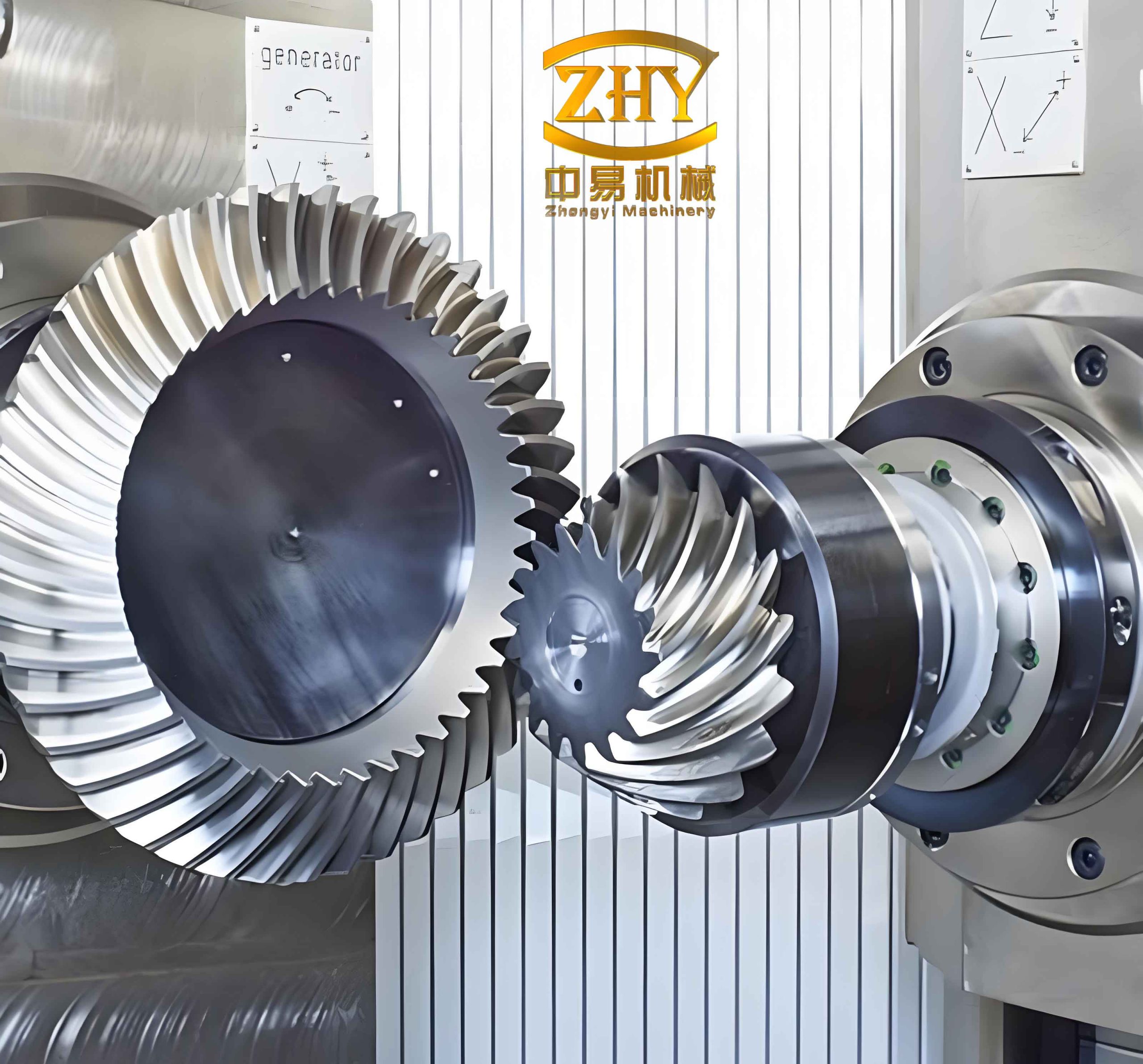
The analytical method I’ve described significantly simplifies the machining process for hyperboloid gears. By reducing the nonlinear equation system to two variables, we can use numerical methods like Newton-Raphson to solve for \( \gamma_1 \) and \( \gamma_2 \). Once these are determined, all other parameters follow directly. This approach minimizes computational effort and enhances accuracy, which is crucial for high-precision applications involving hyperboloid gears.
Moreover, the use of tables and formulas, as shown above, aids in organizing the data and equations. For example, here’s a summary of the iterative solving steps in a procedural format:
| Step | Action | Equations Used |
|---|---|---|
| 1 | Assume initial values for \( \gamma_1 \) and \( \gamma_2 \) | – |
| 2 | Compute \( r_2 \) from large gear dimensions | (7) |
| 3 | Solve for \( r_1 \) using axis distance \( E \) | (3) with approximations |
| 4 | Determine \( e_1 \) and \( e_2 \) from cone geometry | (4) and (5) |
| 5 | Calculate \( \theta_1 \) and \( \theta_2 \) from normal vector conditions | (1) and (2) |
| 6 | Find \( \varepsilon’ \) from generatrix dot product | (9) |
| 7 | Compute \( \psi_1 \) and \( \psi_2 \) using spiral angle relations | (8) and \( \psi_1 = \psi_2 + \varepsilon’ \) |
| 8 | Check if \( r_c \) matches tool curvature and \( \psi_1 \) matches design | (6) and design specs |
| 9 | Adjust \( \gamma_1 \) and \( \gamma_2 \) iteratively until convergence | Numerical methods |
In addition to the core equations, we can derive supplementary formulas for hyperboloid gears. For instance, the relationship between the cone distances and the axis geometry can be expressed as:
$$ L_1 = \frac{r_1}{\sin \gamma_1}, \quad L_2 = \frac{r_2}{\sin \gamma_2} $$
Also, the tooth contact pattern is influenced by the curvature matching. The limit pressure angle \( \phi_0 \) plays a key role in ensuring proper meshing. From equation (6), we see that the tool curvature \( r_c \) must be carefully selected based on the gear parameters to avoid undercutting or excessive wear in hyperboloid gears.
To further elaborate on the machining adjustments, consider the cradle settings. When using a gear generator, the cradle angle \( \alpha_c \) and the machine root angle \( \beta_m \) are critical. They can be derived from the cone angles and spiral angles. For example:
$$ \alpha_c = \gamma_1 + \psi_1 $$
$$ \beta_m = \gamma_2 – \psi_2 $$
These angles ensure that the cutter axis is properly oriented relative to the workpiece. Furthermore, the feed rate and depth of cut must be optimized based on the material and gear size. For hyperboloid gears, which often involve hardened steels, cooling and lubrication are essential to maintain tool life and surface finish.
The advantages of this analytical method are manifold. First, it eliminates the need for complex graphical constructions, reducing human error. Second, it facilitates computer-aided design and manufacturing (CAD/CAM) integration, allowing for automated parameter calculation for hyperboloid gears. Third, it provides a foundation for sensitivity analysis, where we can study how variations in design parameters affect the gear performance. For instance, by taking partial derivatives of equations (1) to (9), we can assess tolerance impacts.
Let me illustrate with a hypothetical example. Suppose we are designing a pair of hyperboloid gears with the following specifications: axis distance \( E = 30 \, \text{mm} \), large gear outer diameter \( D = 100 \, \text{mm} \), face width \( F = 20 \, \text{mm} \), tooth numbers \( N_1 = 20 \) and \( N_2 = 40 \), and desired spiral angles \( \psi_{10} = 30^\circ \) and \( \psi_{20} = 20^\circ \). Using the iterative method, we might find initial guesses for \( \gamma_1 \) and \( \gamma_2 \), say \( \gamma_1 = 20^\circ \) and \( \gamma_2 = 25^\circ \). Then, from (7):
$$ r_2 = \frac{100 – 20 \sin 25^\circ}{2} \approx 45.77 \, \text{mm} $$
From (3), assuming \( \theta_1 \) and \( \theta_2 \) are small initially, we approximate \( r_1 \approx r_2 – E = 15.77 \, \text{mm} \). Then, we proceed through the steps, adjusting \( \gamma_1 \) and \( \gamma_2 \) until convergence. This process can be programmed into software for efficiency.
Another aspect to consider is the manufacturing of hyperboloid gears using modern CNC machines. With the analytical parameters, we can generate tool paths directly. For example, the cutter location data can be computed from the cone equations and adjustment offsets. This enables high-precision machining of hyperboloid gears, which are increasingly used in aerospace and robotics due to their compact design and high torque capacity.
In summary, the machining of hyperboloid gears relies on a deep understanding of their geometric properties. The analytical method I’ve presented simplifies the traditional complex calculations by reducing an 8-variable nonlinear system to a 2-variable one. Through iterative solving and standard machining adjustments, we can accurately produce hyperboloid gears. This approach is not only theoretically sound but also practical for industrial applications. As technology advances, further refinements in algorithms and machine tools will continue to enhance the manufacturing of hyperboloid gears, driving innovation in gear transmission systems.
To reinforce the key points, here is a final table summarizing the benefits of the analytical method for hyperboloid gears:
| Benefit | Description |
|---|---|
| Simplified Calculations | Reduces equation complexity from 8 to 2 variables, easing computation |
| Improved Accuracy | Minimizes errors from graphical methods, leading to precise gear profiles |
| CAD/CAM Integration | Enables seamless data transfer for automated machining of hyperboloid gears |
| Time Efficiency | Accelerates design and adjustment processes, reducing lead times |
| Versatility | Applicable to various hyperboloid gears designs, from automotive to industrial |
| Cost-Effectiveness | Lowers reliance on trial-and-error, saving material and labor costs |
In conclusion, hyperboloid gears are pivotal components in advanced mechanical systems, and their machining demands sophisticated approaches. The analytical method outlined here, with its emphasis on equation simplification and practical adjustments, provides a robust framework for manufacturing these gears. By leveraging mathematical rigor and modern computing, we can overcome the historical challenges associated with hyperboloid gears, paving the way for more efficient and reliable gear transmissions. As I reflect on this topic, it’s clear that continued research and development in this area will further optimize the processes, ensuring that hyperboloid gears meet the evolving demands of engineering applications.