
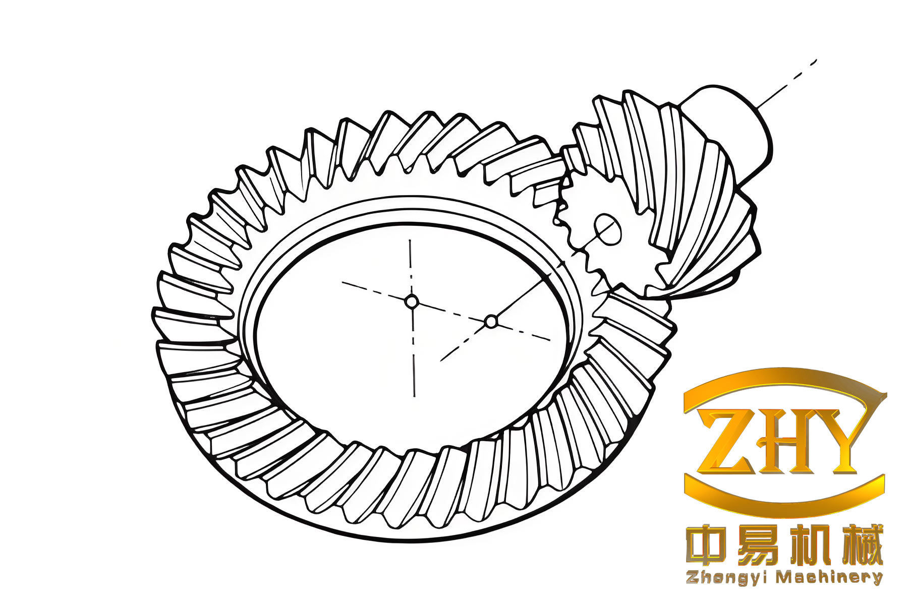
In my research, I focused on hypoid bevel gears because they are widely used in automotive drive axles, especially in main reducers where high transmission ratio, smooth operation, and strong load-carrying capacity are required. Unlike ordinary bevel gears, hypoid bevel gears have a pinion offset relative to the gear axis. This offset increases the pinion diameter, improves the stiffness and strength of the pinion, and allows the whole drive axle to be arranged with a lower floor and a lower center of gravity. At the same time, the tooth surface geometry of hypoid bevel gears is much more complex than that of spur or helical gears. The contact pattern and transmission error are two of the most important indicators of their meshing performance. Poor meshing performance can increase vibration and noise, reduce reliability, and even affect the safety of the drive axle. Therefore, I developed a method that considers both the tooth surface contact pattern and the transmission error, and I also studied how installation errors affect the meshing behavior of hypoid bevel gears.
1. Motivation and Scope
I began with the observation that the traditional design of hypoid bevel gears often relies on local synthesis. In local synthesis, only the neighborhood of a chosen reference point is controlled. This means that the contact pattern and transmission error away from the reference point may not meet the design requirements. In practice, edge contact, an excessively large inclination angle of the contact path, and a discontinuous transmission error curve are frequently observed. These defects reduce the effective contact area, concentrate the load, and increase noise. I therefore set out to build a complete chain from tooth surface modeling to contact analysis, from meshing performance optimization to installation error sensitivity reduction, and finally to cutting and rolling tests.
The main questions I addressed were:
- How can the tooth surfaces of hypoid bevel gears be represented accurately from the cutting process?
- How can the contact pattern and transmission error be computed and evaluated quantitatively?
- How can the machine-tool settings be optimized so that the entire tooth surface, not only a local reference point, has favorable meshing behavior?
- How sensitive is the meshing performance of hypoid bevel gears to different installation errors, and how can this sensitivity be reduced?
- How can the proposed method be verified by cutting, measurement, and rolling inspection?
I use the term hypoid bevel gears repeatedly because the entire study is centered on them. The following sections describe the mathematical models, optimization algorithms, numerical simulations, and experimental validation.
2. Geometric Modeling of Hypoid Bevel Gears
I modeled the hypoid bevel gear tooth surfaces from the cutting process. The machine tool is of the cradle type. The cutter head rotates, and the cutting edges generate a virtual generating gear. The gear blank and the virtual generating gear move relative to each other according to a prescribed ratio. For the gear member, I used a forming method. For the pinion member, I used a tilt method. The tooth surface equations were obtained by coordinate transformation from the cutter coordinate system to the blank coordinate system.
2.1 Cutter Surface and Normal Vector
For the gear cutter, the cutting edge is a straight line. The cutter surface can be written in the cutter coordinate system as:
$$
\mathbf{r}_c(u_c,\theta_c)=
\begin{bmatrix}
(r_d-u_c\sin\alpha_c)\cos\theta_c\\
(r_d-u_c\sin\alpha_c)\sin\theta_c\\
-u_c\cos\alpha_c\\
1
\end{bmatrix}
$$
where \(u_c\) is the generatrix parameter, \(\theta_c\) is the cutter rotation angle, \(r_d\) is the cutter tip radius, and \(\alpha_c\) is the cutter profile angle. The unit normal vector is:
$$
\mathbf{n}_c=
\frac{\frac{\partial \mathbf{r}_c}{\partial u_c}\times
\frac{\partial \mathbf{r}_c}{\partial \theta_c}}
{\left\|\frac{\partial \mathbf{r}_c}{\partial u_c}\times
\frac{\partial \mathbf{r}_c}{\partial \theta_c}\right\|}
=
\begin{bmatrix}
-\cos\alpha_c\cos\theta_c\\
-\cos\alpha_c\sin\theta_c\\
-\sin\alpha_c
\end{bmatrix}
$$
For the gear member, the cutter coordinate system is transformed to the gear blank coordinate system by the machine coordinate system. I can write the gear tooth surface as:
$$
\mathbf{r}_m=\mathbf{M}_{mg}\mathbf{M}_{gc}\mathbf{r}_c,\qquad
\mathbf{n}_m=\mathbf{L}_{mg}\mathbf{L}_{gc}\mathbf{n}_c
$$
For the pinion member, additional tilt and swivel adjustments are required. The cutter surface is transformed through the tilt coordinate system, the swivel coordinate system, the cradle coordinate system, and the blank coordinate system:
$$
\mathbf{r}_p=\mathbf{M}_{pw}\mathbf{M}_{wf}\mathbf{M}_{fu}\mathbf{M}_{uq}\mathbf{M}_{qr}\mathbf{M}_{rA}\mathbf{M}_{Ap}\mathbf{r}_c
$$
$$
\mathbf{n}_p=\mathbf{L}_{pw}\mathbf{L}_{wf}\mathbf{L}_{fu}\mathbf{L}_{uq}\mathbf{L}_{qr}\mathbf{L}_{rA}\mathbf{L}_{Ap}\mathbf{n}_c
$$
The meshing equation between the cutter and the pinion blank is:
$$
\mathbf{n}_q\cdot \mathbf{v}_q=0
$$
where \(\mathbf{n}_q\) is the normal vector in the machine coordinate system and \(\mathbf{v}_q\) is the relative velocity. This equation allows the parameter \(u_p\) to be expressed as a function of \(\theta_p\) and the cradle angle \(\phi_c\):
$$
u_p=u_p(\theta_p,\phi_c)
$$
Substituting this relation into the coordinate transformation gives the final pinion tooth surface equation:
$$
\mathbf{r}_p=\mathbf{r}_p(\theta_p,\phi_c),\qquad
\mathbf{n}_p=\mathbf{n}_p(\theta_p,\phi_c)
$$
2.2 Root Fillet Surface
The root fillet is generated by the tip round corner of the cutter. I included it because the fillet affects the stress concentration and the tooth root strength. For the gear member, the fillet surface can be written as:
$$
\mathbf{r}_e=
\begin{bmatrix}
u_{c0}-r_k\cos\gamma_c+r_k\sin\alpha_c\cos\gamma_c\\
0\\
-r_d-r_k\sin\gamma_c+r_k\cos\alpha_c\cos\gamma_c\\
1
\end{bmatrix}
$$
After transformation to the blank coordinate system, the root fillet surface and its normal vector are:
$$
\mathbf{r}_{mf}=\mathbf{M}_{cg}\mathbf{M}_{gm}\mathbf{r}_e,\qquad
\mathbf{n}_{mf}=\mathbf{L}_{cg}\mathbf{L}_{gm}\mathbf{n}_e
$$
For the pinion, the fillet surface has one more parameter because the blank rotates during cutting. The same transformation chain is used, but the rotational angle of the blank is retained as an independent parameter.
2.3 Discretization and Three-Dimensional Model
I discretized the tooth surface by projecting it onto the axial section. The projection boundary is defined by the outer cone, the inner cone, the addendum, and the dedendum. I used a \(5\times 9\) grid, which gives 45 discrete points for each tooth surface. The mapping between the spatial tooth surface and the projection plane is:
$$
x_P=x(u_c,\theta_c)
$$
$$
y_P=\sqrt{y^2(u_c,\theta_c)+z^2(u_c,\theta_c)}
$$
For each grid point, I solved the nonlinear equations by using the parameters of the neighboring point as the initial guess. The solution path was planned from the center of the projection grid outward, which improved convergence. The resulting point cloud was imported into a computer-aided design environment, and a fitted surface was generated. Boolean operations between the fitted surface and the blank produced one tooth slot. A circular pattern then produced the complete three-dimensional model of the hypoid bevel gears.
| Parameter | Pinion | Gear |
|---|---|---|
| Hand of spiral | Left | Right |
| Number of teeth | 9 | 39 |
| Face width (mm) | 59.25 | 54.00 |
| Spiral angle (deg) | 48.36 | 36.54 |
| Offset (mm) | 35.00 | |
| Whole tooth depth (mm) | 17.07 | 16.90 |
| Pitch cone angle (deg) | 15.65 | 74.01 |
| Face cone angle (deg) | 19.60 | 76.30 |
| Root cone angle (deg) | 14.95 | 70.57 |
| Outer cone distance (mm) | 97.19 | 84.72 |
The table above summarizes the blank parameters I used in the numerical example. These parameters were used consistently in the contact analysis, optimization, simulation, and experiments.
3. Tooth Contact Analysis of Hypoid Bevel Gears
Tooth contact analysis is the core of my theoretical work. I built a virtual assembly coordinate system for the gear pair. The gear and pinion tooth surfaces were transformed into the same meshing coordinate system. At a contact point, the position vectors and the unit normal vectors of the two surfaces must be equal:
$$
\mathbf{r}_m^{(T)}=\mathbf{r}_w^{(T)},\qquad
\mathbf{n}_m^{(T)}=\mathbf{n}_w^{(T)}
$$
For the initial contact point, I chose the midpoint of the gear tooth surface. The corresponding point on the pinion was found by solving the nonlinear contact equations. The unknown variables were the gear rotation angle, the pinion rotation angle, and the pinion surface parameters. After the initial point was determined, I rotated the pinion in small increments and solved the contact equations again. The resulting contact points formed the contact path. The contact ellipses at these points formed the contact pattern.
3.1 Contact Ellipse and Curvature Relations
The contact ellipse is determined by the induced normal curvature and the induced geodesic torsion. For the gear, the normal curvatures along the tooth length and tooth height directions and the geodesic torsion are:
$$
k_{1m}=-\frac{\cos\alpha_c}{r_d-u_c\sin\alpha_c}
$$
$$
k_{2m}=\frac{\sin\alpha_c}{r_d-u_c\sin\alpha_c}
$$
$$
k_{3m}=0
$$
For the pinion, the corresponding curvature parameters in the meshing coordinate system are obtained by rotating the principal directions. If the angle between the pinion principal direction and the gear tooth length direction is \(\theta_0\), then:
$$
k_{1w}^{0}=k_{1w}\cos^2\theta_0+k_{2w}\sin^2\theta_0-2k_{3w}\sin\theta_0\cos\theta_0
$$
$$
k_{2w}^{0}=k_{1w}\sin^2\theta_0+k_{2w}\cos^2\theta_0+2k_{3w}\sin\theta_0\cos\theta_0
$$
$$
k_{3w}^{0}=(k_{1w}-k_{2w})\sin\theta_0\cos\theta_0+k_{3w}(\cos^2\theta_0-\sin^2\theta_0)
$$
The induced curvatures are:
$$
k_1^{0}=k_{1m}-k_{1w}^{0}
$$
$$
k_2^{0}=k_{2m}-k_{2w}^{0}
$$
$$
k_3^{0}=k_{3m}-k_{3w}^{0}
$$
The relative normal curvature in any direction \(\beta\) on the common tangent plane is:
$$
\Delta K=k_1^{0}\cos^2\beta+k_2^{0}\sin^2\beta+2k_3^{0}\sin\beta\cos\beta
$$
The directions of the maximum and minimum relative normal curvatures are:
$$
\Delta K_{\max}=\frac{k_1^{0}+k_2^{0}}{2}
+\sqrt{\left(\frac{k_1^{0}-k_2^{0}}{2}\right)^2+(k_3^{0})^2}
$$
$$
\Delta K_{\min}=\frac{k_1^{0}+k_2^{0}}{2}
-\sqrt{\left(\frac{k_1^{0}-k_2^{0}}{2}\right)^2+(k_3^{0})^2}
$$
The semi-major and semi-minor axes of the contact ellipse are:
$$
l_{\max}=\sqrt{\frac{2\delta}{|\Delta K_{\min}|}},\qquad
l_{\min}=\sqrt{\frac{2\delta}{|\Delta K_{\max}|}}
$$
where \(\delta\) is the equivalent thickness of the marking compound. In my calculation, I used \(\delta=0.00635\) mm, which is a common value in rolling inspection.
3.2 Transmission Error
The transmission error is defined as the difference between the actual gear rotation and the theoretical rotation for a given pinion rotation:
$$
\Delta \varepsilon=\phi_w-\frac{z_1}{z_2}\phi_m
$$
where \(\phi_w\) is the actual gear rotation angle, \(\phi_m\) is the pinion rotation angle, \(z_1\) is the pinion tooth number, and \(z_2\) is the gear tooth number. I plotted the transmission error as a function of the pinion rotation. For a well-designed hypoid bevel gear pair, the transmission error curve should be concave downward, and adjacent curves should intersect. The intersection means that one pair of teeth leaves contact while the next pair enters contact, which gives smooth transmission.
| Quality indicator | Undesirable condition | Effect |
|---|---|---|
| Contact position | Toe, heel, top, or root contact | Load concentration and edge contact |
| Contact size | Too short, too long, too narrow, or too wide | Poor load sharing and high stress |
| Contact shape | Diamond or hard mark | Unstable meshing and noise |
| Transmission error | No intersection or upward curve | Vibration and impact |
In my initial design, the contact pattern of the hypoid bevel gears had edge contact, the inclination angle of the contact path was too large, and the transmission error curve was discontinuous. These defects motivated the optimization described in the next section.
4. Meshing Performance Optimization
I formulated the optimization problem by considering three objectives: the contact area \(S\), the inclination angle \(\gamma\) of the contact path, and the ordinate \(\delta\) of the intersection point of the transmission error curve. The objective function was:
$$
f(S,\gamma,\delta)=
\frac{|S-S_1|}{\varepsilon_1}
+\frac{|\gamma-\gamma_1|}{\varepsilon_2}
+\frac{|\delta-\delta_1|}{\varepsilon_3}
$$
where \(S_1\), \(\gamma_1\), and \(\delta_1\) are the target values, and \(\varepsilon_1\), \(\varepsilon_2\), and \(\varepsilon_3\) are the desired accuracies. I minimized this function by adjusting the machine-tool settings of the pinion. The gear machine-tool settings were kept unchanged because the gear is larger and its cutting cycle is longer.
4.1 Control Parameters
The contact characteristics are controlled by the induced curvature and the induced geodesic torsion. Instead of directly adjusting all machine-tool settings, I used the pinion pitch cone curvature parameters as control variables. The generating radius \(r_0\), the direction angle \(\omega_0\), and the induced curvature \(k_0\) are related to the pinion curvature parameters \(k_1\), \(k_2\), and \(k_3\):
$$
r_0=\frac{\cos\alpha_f}{k_2}
$$
$$
\omega_0=\arctan\left(\frac{k_3}{k_2}\right)
$$
$$
k_0=\frac{k_1k_2-k_3^2}{k_2}
$$
I defined the search space by scaling the initial values:
$$
k_1\in[(1-a_0)k_1^{0},(1+a_0)k_1^{0}]
$$
$$
k_2\in[(1-b_0)k_2^{0},(1+b_0)k_2^{0}]
$$
$$
k_3\in[(1-c_0)k_3^{0},(1+c_0)k_3^{0}]
$$
with \(a_0,b_0,c_0\in[0.002,0.2]\). Each particle in the swarm represented one combination of \(k_1\), \(k_2\), and \(k_3\). For each particle, I calculated the corresponding pinion machine-tool settings and performed tooth contact analysis.
4.2 Constraints
I constrained the contact pattern to lie within a feasible region on the tooth surface. The feasible region was obtained by shrinking the tooth boundary inward:
$$
H_i=\frac{L_i^{0}}{L_i},\qquad i=1,2
$$
where \(L_1\) and \(L_2\) are the tooth length and tooth width, and \(L_1^{0}\) and \(L_2^{0}\) are the corresponding feasible dimensions. I used \(H_i=0.9\). If a contact ellipse extended outside this region, the corresponding particle was removed from the swarm. This prevented edge contact under load.
4.3 Improved Particle Swarm Optimization
I used an improved particle swarm optimization algorithm. In the standard algorithm, the velocity and position updates are:
$$
V_i^{t+1}=V_i^{t}+c_1r_1(P_{ibest}^{t}-X_i^{t})+c_2r_2(G_{best}^{t}-X_i^{t})
$$
$$
X_i^{t+1}=X_i^{t}+V_i^{t+1}
$$
I replaced the fixed inertia weight with an adaptive inertia weight:
$$
\omega(t)=\omega_{start}-(\omega_{start}-\omega_{end})
\tan\left(0.785\left(1-\left(\frac{t}{t_{\max}}\right)^k\right)\right)
$$
with \(\omega_{start}=0.9\), \(\omega_{end}=0.4\), and \(k=0.6\). The velocity update became:
$$
V_i^{t+1}=\omega(t)V_i^{t}+c_1r_1(P_{ibest}^{t}-X_i^{t})
+c_2r_2(G_{best}^{t}-X_i^{t})
$$
I also introduced the Metropolis criterion from simulated annealing. If a new solution was worse than the current best, it was accepted with probability:
$$
P=\exp\left(\frac{\Delta f}{T}\right)
$$
where \(\Delta f=f_{best}-f_{new}\) and \(T\) is the annealing temperature. This helped the swarm escape local optima. The optimization converged after 36 iterations. The objective function value was 0.016703.
| Quantity | Before optimization | Target | After optimization |
|---|---|---|---|
| Contact area \(S\) (mm\(^2\)) | 153.7528 | 180 | 179.631 |
| Contact path inclination \(\gamma\) (deg) | 46.18 | 25 | 25.221 |
| Intersection ordinate \(\delta\) (rad) | — | \(5\times10^{-5}\) | \(5.029\times10^{-5}\) |
The optimized contact pattern no longer had edge contact. The contact path inclination was reduced, and the transmission error curve had a clear intersection. I then verified the result by finite element contact simulation.
5. Finite Element Contact Simulation
I imported the three-dimensional assembly of the hypoid bevel gears into a finite element environment. The material was 20CrMnTi. The material properties are listed in the table below.
| Property | Value |
|---|---|
| Elastic modulus | 207 GPa |
| Poisson’s ratio | 0.25 |
| Density | 7800 kg/m\(^3\) |
The contact between the tooth surfaces was defined as frictional contact with a friction coefficient of 0.06. The overall mesh size was set to the default value, while the contact surfaces were refined to 0.25 mm. The pinion was the driving member. I released the tangential degree of freedom at the pinion bore and constrained the other directions. A torque of 100 N·m was applied to the pinion. The gear was fixed at its bore. The simulation was performed at several rotation positions, and the contact marks were integrated over one meshing cycle.
| Simulation setting | Value |
|---|---|
| Contact type | Frictional |
| Friction coefficient | 0.06 |
| Contact surface mesh size | 0.25 mm |
| Pinion torque | 100 N·m |
| Gear constraint | Fixed bore |
| Pinion constraint | Tangential release, other directions constrained |
The simulation showed that the optimized hypoid bevel gears had a contact pattern that was more centered and more extended along the tooth length. The edge contact that existed before optimization disappeared. The simulation results agreed with the theoretical tooth contact analysis.
6. Installation Error Analysis
In real assembly, installation errors are unavoidable. I considered four types: gear axial error \(\Delta J\), pinion axial error \(\Delta H\), offset error \(\Delta V\), and shaft angle error \(\Delta \psi\). I introduced these errors into the meshing coordinate transformation. The position vector and normal vector of the gear in the meshing coordinate system became:
$$
\mathbf{r}_m^{(T)}=
\mathbf{M}_{mT}\mathbf{M}_{E}\mathbf{M}_{\psi}\mathbf{M}_{J}
\mathbf{r}_m
$$
$$
\mathbf{n}_m^{(T)}=
\mathbf{L}_{mT}\mathbf{L}_{E}\mathbf{L}_{\psi}\mathbf{L}_{J}
\mathbf{n}_m
$$
For the pinion, the transformation included the pinion axial error:
$$
\mathbf{r}_w^{(T)}=
\mathbf{M}_{wT}\mathbf{M}_{H}\mathbf{r}_w
$$
$$
\mathbf{n}_w^{(T)}=
\mathbf{L}_{wT}\mathbf{L}_{H}\mathbf{n}_w
$$
The contact equations remained:
$$
\mathbf{r}_m^{(T)}=\mathbf{r}_w^{(T)},\qquad
\mathbf{n}_m^{(T)}=\mathbf{n}_w^{(T)}
$$
I varied each installation error within a specified range while keeping the other errors at zero. The ranges were \([-0.5,0.5]\) mm for the axial and offset errors and \([-0.17,0.17]\) deg for the shaft angle error. I then calculated the contact pattern parameters and the transmission error.
| Error type | Gear contact path shift | Pinion contact path shift |
|---|---|---|
| \(\Delta J>0\) | Toward heel and root | Toward heel and top |
| \(\Delta J<0\) | Toward toe and top | Toward toe and root |
| \(\Delta H>0\) | Toward toe and top | Toward toe and root |
| \(\Delta H<0\) | Toward heel and root | Toward heel and top |
| \(\Delta V>0\) | Toward toe and top | Toward toe and root |
| \(\Delta V<0\) | Toward heel and root | Toward heel and top |
| \(\Delta \psi>0\) | Toward toe and top | Toward toe and root |
| \(\Delta \psi<0\) | Toward heel and root | Toward heel and top |
I found that the offset error had the strongest influence on the contact pattern and transmission error of the hypoid bevel gears. The gear axial error had the weakest influence. The contact area and the contact path inclination were more sensitive to installation errors than the centroid coordinates.
7. Sensitivity Optimization for Installation Errors
I defined the sensitivity coefficient of a contact pattern parameter with respect to an installation error as:
$$
F_i=\frac{\Delta f_i}{\Delta e},\qquad i=S,x,y,\gamma
$$
where \(\Delta f_i\) is the change in the contact pattern parameter and \(\Delta e\) is the change in the installation error. The comprehensive sensitivity of a parameter was the sum of its sensitivities to the four error types:
$$
S_S=\frac{\Delta S}{\Delta J}+\frac{\Delta S}{\Delta H}
+\frac{\Delta S}{\Delta V}+\frac{\Delta S}{\Delta \psi}
$$
$$
S_x=\frac{\Delta x}{\Delta J}+\frac{\Delta x}{\Delta H}
+\frac{\Delta x}{\Delta V}+\frac{\Delta x}{\Delta \psi}
$$
$$
S_y=\frac{\Delta y}{\Delta J}+\frac{\Delta y}{\Delta H}
+\frac{\Delta y}{\Delta V}+\frac{\Delta y}{\Delta \psi}
$$
$$
S_\gamma=\frac{\Delta \gamma}{\Delta J}+\frac{\Delta \gamma}{\Delta H}
+\frac{\Delta \gamma}{\Delta V}+\frac{\Delta \gamma}{\Delta \psi}
$$
Because the parameters have different units, I converted the shaft angle error into an equivalent linear error by multiplying it by the mean cone distance. I then constructed a weighted objective function:
$$
\min f(S,x,y,\gamma)=a_1S_S+a_2S_x+a_3S_y+a_4S_\gamma
$$
subject to:
$$
a_1+a_2+a_3+a_4=1
$$
Based on the sensitivity analysis, I selected \(a_1=5/12\), \(a_2=1/4\), \(a_3=1/12\), and \(a_4=1/4\). The control variables were again the pinion pitch cone curvature parameters \(k_1\), \(k_2\), and \(k_3\). The improved particle swarm optimization was used to minimize the weighted sensitivity.
| Contact pattern parameter | \(\Delta J\) | \(\Delta H\) | \(\Delta V\) | \(\Delta \psi\) |
|---|---|---|---|---|
| \(S_S\) before | 22.568 | 8.619 | 10.076 | 13.352 |
| \(S_x\) before | 4.168 | 5.795 | 12.863 | 8.085 |
| \(S_y\) before | 0.612 | 2.543 | 3.258 | 2.671 |
| \(S_\gamma\) before | 4.956 | 6.521 | 13.258 | 4.938 |
| \(S_S\) after | 20.463 | 8.809 | 10.268 | 11.670 |
| \(S_x\) after | 4.301 | 5.186 | 11.725 | 7.558 |
| \(S_y\) after | 0.591 | 2.401 | 3.296 | 2.622 |
| \(S_\gamma\) after | 4.566 | 5.896 | 11.607 | 5.033 |
After optimization, the sensitivity coefficients generally decreased. The largest reduction in sensitivity to the gear axial error was 9.33%, to the pinion axial error was 10.51%, to the offset error was 12.5%, and to the shaft angle error was 12.6%. Although a few coefficients increased because of the coupling among parameters, the overall sensitivity of the hypoid bevel gears to installation errors was reduced.
| Error type | Maximum reduction after optimization |
|---|---|
| Gear axial error \(\Delta J\) | 9.33% |
| Pinion axial error \(\Delta H\) | 10.51% |
| Offset error \(\Delta V\) | 12.5% |
| Shaft angle error \(\Delta \psi\) | 12.6% |
8. Experimental Validation
I validated the proposed method by cutting tests, tooth surface error measurement, and rolling inspection. The gear was cut by a forming method. The pinion was cut by a tilt method. The pinion was machined in three steps: rough cutting, concave finish cutting, and convex finish cutting. The gear was machined by a two-step process: rough cutting and finish lapping. The machine-tool settings before and after optimization were used separately.
8.1 Tooth Surface Measurement
I measured the tooth surfaces on a gear measuring instrument using a \(5\times9\) point grid. The maximum deviations were 0.0092 mm for the convex surface and 0.0088 mm for the concave surface. The required accuracy was 0.01 mm, so the cut hypoid bevel gears met the design requirements.
| Surface | Maximum deviation (mm) | Requirement (mm) | Result |
|---|---|---|---|
| Pinion convex | 0.0092 | 0.01 | Accepted |
| Pinion concave | 0.0088 | 0.01 | Accepted |
8.2 Rolling Inspection
I performed rolling inspection on a semi-automatic bevel gear rolling tester. The gear and pinion were mounted at the specified positions. A marking compound with an equivalent thickness of 0.00635 mm was applied to the teeth. The tester was run for 30 s. The contact marks were then observed and compared with the theoretical results.
Before optimization, the contact pattern showed edge contact, a large inclination angle, and a short distribution along the tooth length. After optimization, the contact pattern was more extended along the tooth length, the inclination angle was smaller, the contact area was larger, and no edge contact occurred. The experimental contact pattern matched the theoretical calculation, which confirmed the effectiveness of the optimization of the hypoid bevel gears.
| Contact feature | Before optimization | After optimization |
|---|---|---|
| Edge contact | Present | Absent |
| Contact path inclination | Large | Reduced |
| Contact distribution along tooth length | Short | Longer |
| Contact area | Smaller | Larger |
8.3 Noise Measurement
I measured the transmission noise during rolling inspection. Ten readings were taken at different times, and the average value was used as the noise level. The average noise before optimization was 69.3 dB. After optimization, the average noise was 59.9 dB. The reduction was 13.6%. This indicates that the optimized hypoid bevel gears had smoother transmission and lower vibration.
| Condition | Average noise (dB) | Reduction |
|---|---|---|
| Before optimization | 69.3 | — |
| After optimization | 59.9 | 13.6% |
I also examined the effect of offset error in the rolling inspection. When the offset error was negative, the contact pattern moved toward the heel and the inclination angle increased. When the offset error was positive, the contact pattern moved toward the toe and the inclination angle decreased. These observations agreed with the theoretical model for installation error sensitivity of hypoid bevel gears.
9. Discussion
The results show that the meshing performance of hypoid bevel gears can be improved by optimizing the pinion machine-tool settings through the pitch cone curvature parameters. The proposed method controls the entire tooth surface rather than only a local reference point. The contact area becomes larger, the contact path inclination becomes more suitable, and the transmission error curve becomes continuous. The installation error sensitivity is also reduced, which means that the optimized hypoid bevel gears can tolerate a certain amount of assembly error without losing favorable meshing behavior.
I found that the offset error is the most important installation error for the hypoid bevel gears in this study. Therefore, in practical assembly, the offset should be controlled with particular care. The gear axial error is less influential, but it still affects the contact pattern. The weighted sensitivity model provides a systematic way to balance different contact pattern parameters and different error types.
The finite element simulation and the rolling inspection both confirmed the theoretical predictions. The maximum tooth surface deviation was within the required tolerance. The noise reduction of 13.6% is significant for automotive drive axle applications. This supports the practical value of the proposed optimization method for hypoid bevel gears.
10. Conclusions
I can summarize my work on hypoid bevel gears as follows:
- I established the tooth surface equations of hypoid bevel gears from the cutting process, including the gear surface, the pinion surface, and the root fillet surface. I solved the equations numerically and built accurate three-dimensional models.
- I constructed a tooth contact analysis model for hypoid bevel gears. I calculated the contact path, contact ellipse, contact pattern, and transmission error. I identified edge contact, large contact path inclination, and discontinuous transmission error as the main defects of the initial design.
- I proposed a meshing performance optimization method that considers both the contact pattern and the transmission error. I used the pinion pitch cone curvature parameters as control variables and an improved particle swarm optimization algorithm with adaptive inertia weight and the Metropolis criterion. The optimized hypoid bevel gears had a larger contact area, a smaller contact path inclination, and a continuous transmission error curve.
- I introduced installation errors into the meshing model. I quantified the sensitivity of the contact pattern parameters to gear axial error, pinion axial error, offset error, and shaft angle error. The offset error was the most influential. I built a weighted sensitivity objective function and optimized the pinion machine-tool settings to reduce the sensitivity of hypoid bevel gears to installation errors.
- I performed cutting tests, tooth surface measurement, and rolling inspection. The experimental results showed that the optimized hypoid bevel gears had no edge contact, a more reasonable contact pattern, and a 13.6% reduction in transmission noise.
Overall, my study provides a complete workflow for the contact characteristic analysis and meshing performance optimization of hypoid bevel gears. The method can be used to improve load distribution, reduce vibration and noise, and increase the tolerance of hypoid bevel gears to installation errors. In future work, I plan to extend the model to loaded contact analysis, multiple simultaneous installation errors, and dynamic meshing behavior.