
In the manufacturing of hypoid gears, achieving the prescribed contact pattern and flank geometry is paramount for ensuring smooth operation, high load capacity, and minimal noise. Traditional full-formate methods, while effective, can introduce theoretical errors when the tool pressure angle differs significantly from the desired root angle of the gear, particularly for the large member (gear). This necessitates the use of machines with a cutter tilt mechanism and an adjusted calculation methodology to directly generate the correct tooth surfaces. This article, from a first-person engineering perspective, details a comprehensive adjustment calculation method for the full-formate cutting of hypoid gears using cutter tilt, designed to eliminate inherent theoretical errors and accelerate the setup process for superior meshing quality.
The core challenge lies in aligning the calculated reference point for gear generation with the desired contact pattern center on the actual tooth flank.
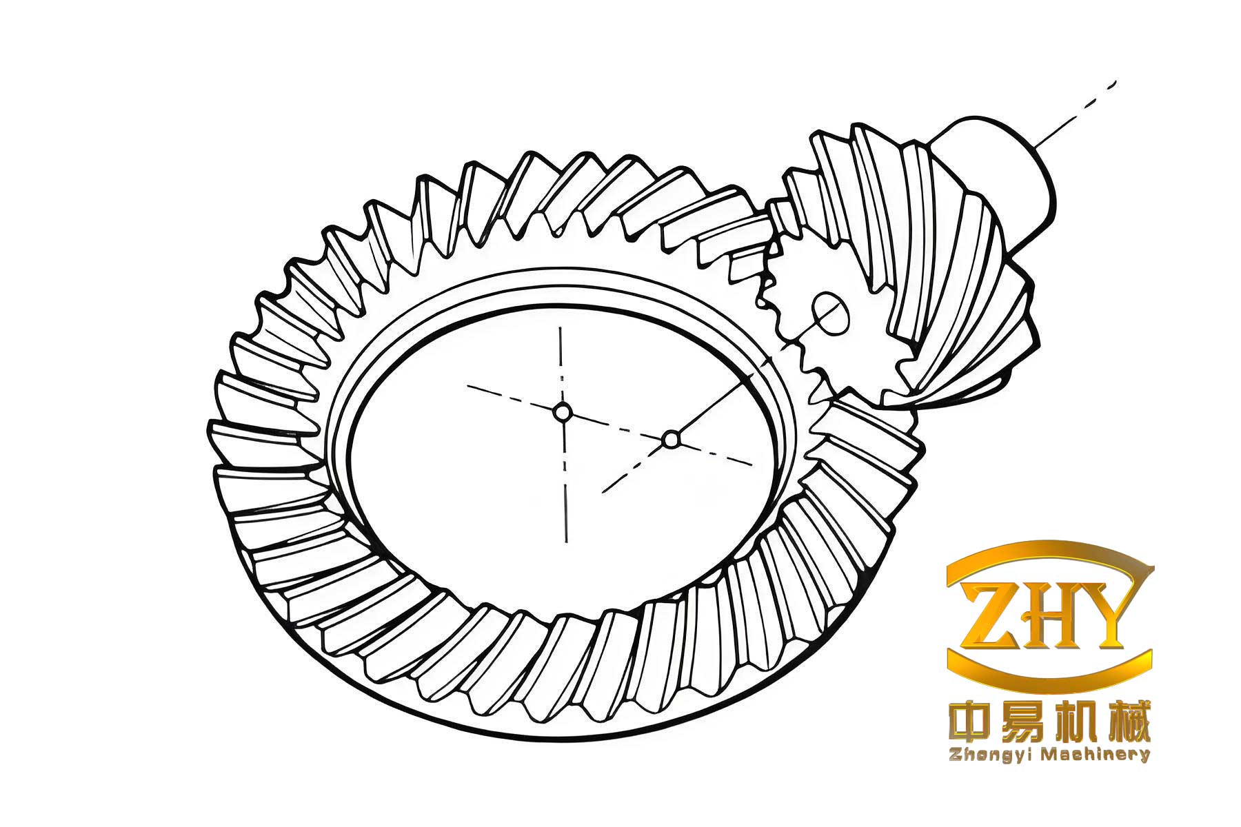
Previous methods often selected a reference point on the mid-point of the gear tooth space, which does not inherently coincide with the contact center. This discrepancy forces machinists to rely on time-consuming trial-and-error adjustments based on actual contact marks. The methodology presented here, which we can term the Cutter Tilt Full-Formate (CTFF) method, allows for the selection of any corresponding point on the mating gear’s flank—typically the contact pattern center—as the computational reference point for generating the pinion. This fundamental shift eliminates the theoretical error at its source.
The foundation of this analysis rests on the study of conjugate surfaces. Instead of analyzing the real gear tooth surfaces directly, we examine two imaginary generating gears and a imaginary crown gear (or plane generating gear) that have “equidistant conjugate surfaces” offset by the cutter point radius from the actual surfaces. The geometry is defined relative to a reference point \( P’_0 \). For the large hypoid gear (Gear 2), the imaginary generating gear \( z’_2 \) shares the same axis and equidistant surface \( \Sigma_2 \) with the real gear, but possesses a different pitch cone. The root cone angle requirement is met by ensuring the pitch plane of the imaginary crown gear \( z_0 \) is tangent to the pitch cones of the imaginary generating gears \( z’_1 \) and \( z’_2 \).
Machine Adjustment Calculation for Finishing the Large Hypoid Gear
The initial step involves determining the machine settings for finishing Gear 2. The spiral angle \( \beta_0 \) and pitch radius \( r_0 \) of the imaginary crown gear \( z_0 \) are calculated by equating its limiting pressure angle \( \alpha_{0L} \) and limiting normal curvature \( k_{0L} \) to those of the imaginary generating gear pair \( z’_1 \) and \( z’_2 \) at their reference point. The formulas are as follows:
$$ \sin \beta_0 = \frac{\sin \alpha’_{0L} \sin \beta’_2}{\sin \alpha_{0L}} $$
$$ r_0 = \frac{\cos \alpha’_{0L} \cos \beta’_2}{\cos \alpha_{0L} \cos \beta_0} \cdot r’_2 $$
Where \( \alpha’_{0L} \) and \( \beta’_2 \) are parameters of the imaginary generating gear \( z’_2 \). Once \( \beta_0 \) and \( r_0 \) are known, key machine settings for Gear 2 can be computed. The vertical offset of the gear, \( V_2 \), and the machine ratio, \( i_{02} \), are given by:
$$ V_2 = r_0 \sin \beta_0 – r’_2 \sin \beta’_2 $$
$$ i_{02} = \frac{r’_2 \cos \beta’_2}{r_0 \cos \beta_0} $$
The sign convention for \( V_2 \) is crucial: positive for left-hand Gear 2 offset below the cradle center, and for right-hand Gear 2 offset above. The pressure angle \( \alpha’_2 \) at point \( P’_0 \) on the imaginary generating gear is calculated from the specified sum of pinion and gear pressure angles \( \alpha_1 + \alpha_2 \). A discrepancy arises because the actual cutter blade angle \( \alpha_{c2} \) is fixed and may not equal \( \alpha’_2 \). To correct the pressure angle error \( \Delta \alpha_2 = \alpha_{c2} – \alpha’_2 \), the cutter axis is tilted. The required tilt adjustments—cutter tilt angle \( I \) and cutter rotation angle \( J \)—are determined alongside corrections to the machine center \( \Delta X_{B2} \) and the sliding base setting \( \Delta X_{D2} \). The formulas involve the mean cutter point radius \( r_{c2} \) and the pitch angle \( \theta_{c2} \):
$$ \Delta X_{B2} = -r_{c2} \Delta \alpha_2 \sin \theta_{c2} $$
$$ \Delta X_{D2} = r_{c2} \Delta \alpha_2 \cos \theta_{c2} $$
The values for \( I \) and \( J \) are selected from a standard table based on the face of the gear being cut (convex or concave) and the hand of spiral. A critical parameter is the distance \( S_{B2} \) from the tilt center to the plane perpendicular to the cradle axis, calculated as:
$$ S_{B2} = \frac{\Delta X_{D2} + q_2 \sin I \cos J}{\cos I} $$
Where \( q_2 \) is the basic machine constant (e.g., 114.591 mm for Gleason No. 116). Finally, the machine center to back, \( X_{B2} \), is found from the geometric relationship: \( X_{B2} = X_{BP2} – S_{B2} \), where \( X_{BP2} \) is a fixed machine dimension.
| Parameter | Symbol | Formula/Note |
|---|---|---|
| Machine Center to Back | \( X_{B2} \) | \( X_{BP2} – S_{B2} \) |
| Machine Center Correction | \( \Delta X_{B2} \) | \( -r_{c2} \Delta \alpha_2 \sin \theta_{c2} \) |
| Vertical Gear Offset | \( V_2 \) | \( r_0 \sin \beta_0 – r’_2 \sin \beta’_2 \) |
| Radial Cutter Distance | \( S_{r2} \) | \( r_0 \) (Nominal) |
| Cutter Tilt Angle | \( I \) | From Standard Table |
| Cutter Rotation Angle | \( J \) | From Standard Table |
| Machine Ratio | \( i_{02} \) | \( \frac{r’_2 \cos \beta’_2}{r_0 \cos \beta_0} \) |
Position of the Contact Point on the Equidistant Conjugate Surface
The pivotal advancement of the CTFF method is shifting the computational reference from the midpoint \( P’_0 \) to the desired contact point \( M \) on the equidistant surface \( \Sigma_2 \) of the large hypoid gear. This point \( M \) corresponds to the center of the target contact pattern. The shift is defined by two increments: \( \Delta R_{2e} \) along the tooth height (positive towards the root) and \( \Delta L_{2e} \) along the pitch cone element (positive towards the toe). If the contact center is at the mid-height, \( \Delta R_{2e} = 0 \). The coordinates of \( M \) in the gear coordinate system are:
$$ R_{2M} = R’_{2P} – \Delta R_{2e} \sin \delta’_2 $$
$$ L_{2M} = L’_{2P} – \Delta L_{2e} $$
Where \( R’_{2P}, L’_{2P}, \delta’_2 \) are coordinates and pitch angle at \( P’_0 \). Through a series of coordinate transformations from the gear system to the stationary machine system and then to the cradle system, we establish the vector equation of the cutter surface \( \Sigma_c \) (a cone) and its unit normal. The condition for conjugation between the cutter surface \( \Sigma_c \) and the gear’s equidistant surface \( \Sigma_2 \) at point \( M \) is that their relative velocity is perpendicular to the common normal. This leads to a system of nonlinear equations that can be solved iteratively (e.g., using Newton’s method) to find the cradle rotation angle \( \phi \) and the parameter \( u \) defining the point on the cutter edge that contacts \( M \).
Once \( M \) is determined in space and its corresponding cradle angle \( \phi_M \) is found, a new imaginary crown gear \( z_{0M} \) and a new imaginary generating gear \( z’_{2M} \) are defined, having \( M \) as their reference point. Their pitch cone parameters \( \delta’_{2M}, \beta’_{2M}, r’_{2M}, etc. \), are calculated. This forms the basis for accurately generating the mating pinion.
Mathematical Modeling for Pinion Generation
With the geometry established for the large hypoid gear at the contact point \( M \), we now focus on generating the pinion (Gear 1). The goal is to calculate the machine settings so that its equidistant surface \( \Sigma_1 \) closely matches the conjugate of \( \Sigma_2 \) at \( M \) and in its immediate vicinity. This requires calculating the curvatures of \( \Sigma_2 \) at \( M \).
The principal curvatures of the cutter surface \( \Sigma_c \) at the contact point are known. Transforming these into the cradle coordinate system and then to the direction of the imaginary crown gear’s tooth line gives us the normal curvature \( k_{0M}^{(\lambda)} \), geodesic torsion \( \tau_{0M}^{(\lambda)} \), and profile direction normal curvature \( k_{0M}^{(t)} \) for the crown gear at \( M \).
The key transfer is using curvature relations (akin to Euler/Savary equations for gear meshing) to find the corresponding curvatures on the imaginary generating gear \( z’_{2M} \). The normal curvature and geodesic torsion of the gear’s equidistant surface \( \Sigma_2 \) along the tooth line direction \( \vec{v}^{(\lambda)} \) at \( M \) are given by:
$$ k_{2M}^{(\lambda)} = \frac{ k_{0M}^{(\lambda)} – 2 k_{sM} \cos \alpha_{cM} + k_{sM}^2 / k_{0M}^{(t)} }{ \sin^2 \alpha_{cM} } $$
$$ \tau_{2M}^{(\lambda)} = \frac{ \tau_{0M}^{(\lambda)} }{ \sin \alpha_{cM} } $$
Here, \( k_{sM} = \frac{\sin \alpha_{cM}}{r_{c2}} \) is related to the cutter radius, and \( \alpha_{cM} \) is the pressure angle at the contact point \( M \). The profile direction normal curvature \( k_{2M}^{(t)} \) is calculated using a separate curvature relation formula. To achieve a favorable contact pattern, a profile curvature modification is often introduced. This is controlled by a modification coefficient \( C_k \), which adjusts the calculated \( k_{2M}^{(t)} \) before proceeding to pinion generation calculations: \( k_{2M}^{(t)}_{mod} = C_k \cdot k_{2M}^{(t)} \).
These curvature values \( (k_{2M}^{(\lambda)}, \tau_{2M}^{(\lambda)}, k_{2M}^{(t)}_{mod}) \) for the large hypoid gear’s surface at the designated contact point, along with the pitch cone parameters of the imaginary gears \( z’_{1M} \) and \( z’_{2M} \), serve as the direct input for calculating the pinion’s finishing machine settings. The calculation follows a systematic procedure similar to the traditional full-formate method but is now anchored to the correct contact point. This procedure determines the pinion’s machine root angle, cutter tilt/rotation, radial distance, and most importantly, the ratio between the cradle and the pinion’s rotation (the machine ratio, \( i_{01} \)), which fundamentally shapes the pinion flank.
Calculation Examples and Comparative Analysis
To illustrate the impact of the CTFF method, let’s examine calculated machine settings for a sample hypoid gear pair. The following tables compare parameters for finishing the gear and the pinion using different reference points.
Table 1: Finishing Machine Settings for the Large Hypoid Gear (Example)
Cutter: \( D_{c2}=152.4mm, W_2=3.175mm, \alpha_{c2}=20^\circ/18^\circ \)
| No. | Parameter | Symbol | Concave Flank | Convex Flank |
|---|---|---|---|---|
| 1 | Machine Center to Back | \( X_{B2} \) | 168.593 mm | 166.971 mm |
| 2 | Machine Center Correction | \( \Delta X_{B2} \) | 0.028 mm | -0.173 mm |
| 3 | Vertical Gear Offset | \( V_2 \) | -3.631 mm | -3.631 mm |
| 4 | Radial Cutter Distance | \( S_{r2} \) | 103.426 mm | 103.426 mm |
| 5 | Cutter Tilt Angle | \( I \) | 15° | 15° |
| 6 | Cutter Rotation Angle | \( J \) | 295° | 257° |
| 7 | Machine Ratio | \( i_{02} \) | 1.32528 | 1.32528 |
Table 2: Finishing Machine Settings for the Pinion (Small Hypoid Gear)
Demonstrating the effect of different contact point shifts (\( \Delta L_{1e} \)) and profile modification (\( C_k \)).
| Parameter | Symbol | Concave Flank (\(\alpha_{c1}=20^\circ\)) | Convex Flank (\(\alpha_{c1}=-18^\circ\)) | ||||
|---|---|---|---|---|---|---|---|
| Case A | Case B | Case C | Case A | Case B | Case C | ||
| Contact Pt. Shift | \( \Delta L_{1e} \) | 0.0 mm | 0.0 mm | -2.0 mm | 0.0 mm | 0.0 mm | +2.0 mm |
| Cutter Pt. Radius | \( r_{c1} \) | 66.863 mm | 66.876 mm | 68.013 mm | 73.831 mm | 73.854 mm | 75.138 mm |
| Machine Ratio | \( i_{01} \) | 2.4399 | 2.2844 | 2.2544 | 2.4399 | 2.2844 | 2.2544 |
| Vertical Pinion Offset | \( E_{M1} \) | -30.517 mm | -30.747 mm | -30.871 mm | -30.517 mm | -30.747 mm | -30.871 mm |
| Cutter Tilt Angle | \( i_1 \) | 35.0° | 33.0° | 33.0° | 35.0° | 33.0° | 33.0° |
| Cutter Rotation Angle | \( j_1 \) | 24.5° | 25.0° | 26.8° | 335.5° | 335.0° | 333.2° |
| Radial Distance | \( S_{r1} \) | 113.615 mm | 114.223 mm | 114.423 mm | 113.615 mm | 114.223 mm | 114.423 mm |
| Machine Center to Back | \( X_{B1} \) | 181.445 mm | 181.064 mm | 181.268 mm | 178.635 mm | 179.002 mm | 179.122 mm |
The data in Table 2 clearly shows that the calculated machine settings for cutting the pinion vary significantly with the chosen reference point (via \( \Delta L_{1e} \)) and the profile modification coefficient \( C_k \) (different between Case A and B). Parameters like cutter point radius, machine ratio, and tilt angles are all interconnected. Adjusting one to position the contact pattern correctly will inherently change the others. The CTFF method provides a deterministic mathematical framework to calculate this interdependent set of parameters directly from the desired gear geometry and contact location, replacing unreliable empirical trial-and-error.
Conclusion
The successful manufacture of high-performance hypoid gears hinges on precise control over the tooth surface geometry. The Cutter Tilt Full-Formate (CTFF) adjustment calculation method presented here offers a significant refinement over traditional approaches. By explicitly using the desired contact pattern center as the fundamental reference point for all generation calculations, it eliminates the inherent theoretical error present in methods that use a fixed geometric midpoint. This is achieved through a rigorous mathematical process that involves: calculating the machine settings for the large hypoid gear with cutter tilt corrections; determining the exact position and local surface properties (curvatures) at the designated contact point on its flank; and using this data to compute the precise cradle drive ratio, cutter orientation, and positional settings needed to generate the conjugate pinion flank.
The method incorporates essential refinements such as root angle correction for the pinion and controlled profile curvature modification, providing the engineer with direct levers to influence the contact pattern shape and size. As demonstrated in the calculation examples, the resulting machine settings are sensitive to the target contact location, confirming the method’s accuracy. Adopting this methodology allows for a dramatic reduction in setup time on the gear cutting machine, as the initial theoretical setup places the contact pattern very close to its intended location. More importantly, it ensures the resulting hypoid gear pair possesses the optimal meshing characteristics designed into it, leading to improved transmission efficiency, durability, and quiet operation. This systematic approach is vital for the advanced manufacturing of reliable hypoid gear drives.