
In modern manufacturing, the selection of appropriate tooling, including cutting tools, tool holders, and fixtures, is crucial for optimizing resource utilization, enhancing production quality and efficiency, and reducing costs in gear hobbing processes. Gear hobbing, a fundamental method for generating gears, involves complex interactions between the workpiece, machine, and tooling. Traditional tooling selection often relies on operator experience, leading to inconsistencies, inefficiencies, and increased downtime. To address these challenges, I propose an intelligent selection method specifically designed for gear hobbing machine tooling. This method integrates information modeling, rule-based reasoning, and multi-criteria decision-making to automate and optimize the selection process. By leveraging advanced algorithms, it ensures that the most suitable combination of hob, arbor, and fixture is chosen based on real-time shop-floor data and processing requirements, thereby supporting the transition towards smart manufacturing in gear production.
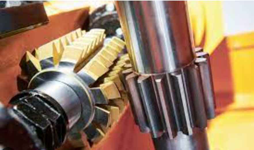
The gear hobbing process is a continuous generating operation where a helical cutting tool, known as a hob, rotates and feeds to cut teeth into a gear blank. This method is widely used for its versatility in producing spur and helical gears. However, the effectiveness of gear hobbing heavily depends on the correct selection of tooling components. Inadequate tooling can result in poor surface finish, dimensional inaccuracies, tool wear, and increased production costs. Current research on tooling selection has primarily focused on general CNC machining, with limited attention to the specialized needs of gear hobbing. Moreover, existing approaches often treat tool selection in isolation, without considering the integrated selection of hobs, arbors, and fixtures as a cohesive system. This gap highlights the need for a comprehensive, intelligent method tailored to gear hobbing machines.
My intelligent selection method for gear hobbing machine tooling consists of three interconnected parts. First, I establish detailed information models and selection rules by analyzing the characteristics of tooling components and the principles of gear hobbing. Second, I develop a preliminary selection model using rule-based reasoning (RBR) to generate a candidate set of tooling that meets basic processing requirements. Third, I apply an optimization decision-making approach based on the Analytic Hierarchy Process (AHP) and Grey Relational Analysis (GRA) to select the optimal tooling combination from the candidate set. This holistic framework ensures that tooling selection is both technically sound and economically viable, adapting dynamically to changing production conditions. Throughout this article, I will elaborate on each part, supported by formulas, tables, and a case study to demonstrate practical applicability.
To begin, I analyze the information features of gear hobbing machine tooling and the machining tasks. In gear hobbing, the processing elements can be categorized into three groups: workpiece requirements, process requirements, and clamping requirements. Accordingly, the machining task information includes workpiece parameters related to workpiece requirements, process parameters related to process requirements, and clamping information related to clamping requirements. The information model for the machining task is summarized in the table below.
| Category | Information Type | Examples |
|---|---|---|
| Workpiece Requirements | Geometric Parameters | Normal module, pressure angle, helix angle, number of teeth |
| Material Properties | Material type, hardness, tensile strength | |
| Quality Specifications | Surface roughness, tolerance grades | |
| Process Requirements | Machining Operations | Roughing, semi-finishing, finishing |
| Process Parameters | Cutting speed, feed rate, depth of cut | |
| Clamping Requirements | Machine Interface | Machine spindle type, arbor mounting dimensions |
| Workpiece Holding | Fixture type, clamping force, locating surfaces |
For the tooling components, I focus on the hob, arbor, and fixture. The hob information is divided into six categories: profile parameters, edge parameters, external parameters, structural parameters, process parameters, and coating material parameters. The arbor and fixture have simpler information sets, primarily related to clamping dimensions and compatibility. The tooling information model is outlined as follows.
| Tooling Component | Information Category | Key Parameters |
|---|---|---|
| Hob | Profile Parameters | Normal module, pressure angle, tooth thickness, addendum, dedendum |
| Edge Parameters | Rake angle, clearance angle, helix angle | |
| External Parameters | Outer diameter, bore diameter, overall length | |
| Structural Parameters | Type (e.g., integral, shell), number of gashes | |
| Process Parameters | Accuracy grade, coating type, application (e.g., pre-grind, finish) | |
| Coating Material | Material (e.g., TiN, TiAlN), thickness | |
| Arbor | Clamping Parameters | Shank diameter, tool mounting diameter, maximum tool length, keyway dimensions |
| Fixture | Clamping Parameters | Clamping method (e.g., chuck, vise), clamping range, locating accuracy |
Based on these models, I derive selection rules for each tooling component. For gear hobbing, the hob selection rules are primarily governed by the generative principle of gear hobbing, where the hob acts as a mating gear. The rules ensure that the hob profile matches the gear to be produced. For example, the normal module of the hob must equal the normal module of the gear. Similarly, the pressure angle must correspond. These rules are expressed mathematically. Let \( m_{n0} \) be the hob normal module, \( m_n \) be the gear normal module, \( \alpha_{n0} \) be the hob normal pressure angle, and \( \alpha_n \) be the gear normal pressure angle. The matching rules are:
$$ m_{n0} = m_n $$
$$ \alpha_{n0} = \alpha_n $$
Other parameters, such as tooth thickness and addendum, are derived from the gear data. For instance, the hob normal tooth thickness \( s_{on} \) is calculated as:
$$ s_{on} = \frac{p_{on}}{2} = \frac{\pi m_n}{2} $$
where \( p_{on} \) is the normal pitch. The axial pitch \( p_{ox} \) considers the helix angle \( \beta \):
$$ p_{ox} = \frac{p_{on}}{\cos \beta} $$
For edge parameters, typical values include a rake angle of 7° to 9° for general purposes, and up to 12° to 15° for roughing. Clearance angles are usually 10° to 12° at the top and 2° to 3° at the sides. The hob hand (right or left) should generally match the gear hand to ensure proper cutting action. The number of starts affects efficiency and accuracy; single-start hobs are preferred for finishing to achieve better surface finish, while multi-start hobs may be used for roughing to increase material removal rates.
The hob structural type selection depends on the application. Shell hobs (with a bore) are common for general use and require an arbor, while shank hobs are used for specialized applications and mount directly to the machine. The accuracy grade of the hob is chosen based on the gear accuracy requirement. For example, for gear quality grades per ISO standards, AA-grade hobs are used for high-precision gears (e.g., grade 6), A-grade for grade 7, B-grade for grade 8, and C-grade for lower grades. Coating material selection relates to cutting speed ranges: high-speed steel (HSS) with coatings like TiN is suitable for speeds up to 50 m/min, while powder metallurgy HSS or carbide is used for higher speeds exceeding 150 m/min.
For the arbor, selection rules focus on compatibility with both the machine and the hob. The arbor shank diameter must match the machine spindle bore diameter, typically with a clearance fit for easy assembly and disassembly. The tool mounting diameter must equal the hob bore diameter, also with a clearance fit. The arbor’s maximum tool length must exceed the hob overall length to ensure secure clamping. Additionally, the keyway width on the arbor must match the hob keyway width to transmit torque effectively. These rules ensure proper power transmission and alignment during gear hobbing.
For the fixture, rules depend on the workpiece geometry. For gear shafts (longitudinal workpieces), chuck-type fixtures are used, often with centers for support. For gear blanks (disk-type workpieces), vise or plate fixtures with screw clamping are employed. The fixture must accommodate the workpiece dimensions within its clamping range. For instance, a chuck with a clamping range of 0–50 mm can hold shafts up to 50 mm in diameter. Proper selection ensures stability and accuracy during machining.
I formalize these rules into a rule base using production rule representation, such as “IF condition THEN conclusion.” For example:
- IF gear normal module = 3 AND gear pressure angle = 20° THEN hob normal module = 3 AND hob pressure angle = 20°.
- IF machine spindle bore = 32 mm AND hob bore = 32 mm THEN arbor shank diameter = 32 mm.
- IF workpiece type = gear shaft AND shaft diameter ≤ 20 mm THEN fixture type = chuck with 0–20 mm range.
With the information models and rules established, I proceed to the second part: developing a preliminary selection model using rule-based reasoning (RBR). RBR is suitable here because the knowledge is explicit and can be easily represented as rules. The inference engine employs forward chaining: starting with the machining task facts, it matches conditions in the rule base to derive conclusions. The process involves:
- Input machining task parameters (e.g., gear data, process requirements) into the fact database.
- Match facts with rule conditions; if a match occurs, the rule is activated.
- Execute activated rules to infer tooling types that satisfy the requirements.
- Check the availability of inferred tooling types in the shop-floor inventory.
- Output a candidate set of tooling types that are both technically suitable and available.
The candidate set includes hobs, arbors, and fixtures. Let \( H \) be the set of candidate hobs, \( B \) the set of candidate arbors, and \( F \) the set of candidate fixtures. The overall candidate tooling set \( T \) is:
$$ T = \{ H, B, F \} $$
Each set is derived through rule application. For hobs, the selection considers multiple constraints: workpiece requirements (e.g., gear geometry), process requirements (e.g., accuracy), and clamping requirements (e.g., hob dimensions). Mathematically, let \( R_H \) be the set of hob selection rules, partitioned into subsets for workpiece requirements \( R_{Hm} \), process requirements \( R_{Hc} \), and clamping requirements \( R_{Hf} \). The candidate hob set \( H \) is the intersection of the sets obtained from applying each rule subset:
$$ H = H_m \cap H_c \cap H_f $$
where \( H_m = F(R_{Hm}) \), \( H_c = F(R_{Hc}) \), \( H_f = F(R_{Hf}) \), and \( F(\cdot) \) denotes the inference function.
Similarly, for arbors, rules focus on clamping compatibility: \( R_B = R_{Bf} \) (clamping requirements only), so:
$$ B = F(R_{Bf}) $$
For fixtures, rules also focus on clamping: \( R_F = R_{Ff} \), so:
$$ F = F(R_{Ff}) $$
If any set is empty, it indicates no suitable tooling is available, triggering a procurement request. Otherwise, the candidate set \( T \) is formed. Importantly, hobs and arbors have a mapping relationship; a hob type may require a specific arbor type. Thus, the candidate hob set \( H \) is filtered to remove hobs without matching arbors in \( B \). This ensures that only feasible combinations are considered.
The selection workflow is as follows: first, select candidate hobs based on gear and process data; second, select candidate arbors based on machine and hob data; third, update the hob set by removing hobs without arbors; fourth, select candidate fixtures based on workpiece clamping data; fifth, compile the candidate tooling set. This systematic approach reduces the search space and ensures compatibility.
To illustrate the candidate set model, suppose after inference, we have \( n \) hob types, \( m \) arbor types, and \( k \) fixture types. Each type has multiple instances in inventory. The candidate set can be visualized as a three-dimensional space with axes for hobs, arbors, and fixtures, where each point represents a tooling instance. However, for selection purposes, we focus on the types and their available quantities. Let \( N_{H_i} \) be the number of available hobs of type \( i \), \( N_{B_j} \) for arbors, and \( N_{F_l} \) for fixtures. The candidate set includes all these instances, but the next step is to choose the optimal combination.
The candidate set from RBR may contain multiple options, so I introduce a decision-making method to identify the best tooling combination. This is the third part of my method, using AHP and GRA. AHP helps determine the relative importance of evaluation criteria, while GRA assesses the similarity between each tooling option and an ideal solution. The criteria are derived from production objectives: machining quality, efficiency, and cost. For gear hobbing, machining quality \( Q \) is influenced by surface roughness \( Ra \) (for hobs) and clamping accuracy (for arbors and fixtures). Machining efficiency \( E \) is related to total processing time, including basic machining time \( t_1 \) (cutting time) and auxiliary time \( t_2 \) (setup and tool change time). Machining cost \( C \) includes tooling usage cost \( c_1 \), machine usage cost \( c_2 \), and energy consumption cost \( c_3 \). These criteria are organized into a hierarchy for AHP.
I apply AHP to assign weights to the criteria. First, I construct a pairwise comparison matrix \( G \) for the criteria. Let the criteria be: \( C_1 \) for quality, \( C_2 \) for efficiency, and \( C_3 \) for cost. Based on expert judgment, I compare their importance. For example, if quality is moderately more important than efficiency, and cost is strongly more important than quality, the matrix might be:
$$ G = \begin{bmatrix} 1 & a_{12} & a_{13} \\ a_{21} & 1 & a_{23} \\ a_{31} & a_{32} & 1 \end{bmatrix} $$
where \( a_{pq} \) represents the relative importance of criterion \( p \) over criterion \( q \). Using Saaty’s scale (1 for equal importance, 3 for moderate, 5 for strong, etc.), suppose \( a_{12} = 1/3 \), \( a_{13} = 1/5 \), \( a_{21} = 3 \), \( a_{23} = 1/2 \), \( a_{31} = 5 \), \( a_{32} = 2 \). Then:
$$ G = \begin{bmatrix} 1 & 1/3 & 1/5 \\ 3 & 1 & 1/2 \\ 5 & 2 & 1 \end{bmatrix} $$
I compute the eigenvector corresponding to the largest eigenvalue to get the weights. The normalized weight vector \( W \) is approximately:
$$ W = \begin{bmatrix} w_1 \\ w_2 \\ w_3 \end{bmatrix} = \begin{bmatrix} 0.105 \\ 0.258 \\ 0.637 \end{bmatrix} $$
after consistency check (consistency ratio < 0.1). Thus, for this example, cost is the most important criterion, followed by efficiency and quality.
Next, for each tooling type (e.g., hobs), I evaluate individual instances using GRA. Suppose we have \( u \) candidate hobs. For each hob, I collect data for the three criteria: quality index (e.g., surface roughness \( Ra \)), efficiency index (total time \( t = t_1 + t_2 \)), and cost index (total cost \( c = c_1 + c_2 + c_3 \)). These form a comparison sequence matrix \( K \):
$$ K = \begin{bmatrix} k_{11} & k_{12} & k_{13} \\ k_{21} & k_{22} & k_{23} \\ \vdots & \vdots & \vdots \\ k_{u1} & k_{u2} & k_{u3} \end{bmatrix} $$
where \( k_{i1} \) is the \( Ra \) value for hob \( i \), \( k_{i2} \) is the total time, and \( k_{i3} \) is the total cost. For quality, lower \( Ra \) is better; for time and cost, lower values are also better. So, I define an ideal reference sequence \( K_0 \) as the best values across all candidates: \( K_0 = [k_{01}, k_{02}, k_{03}] \), where \( k_{01} = \min_i k_{i1} \), \( k_{02} = \min_i k_{i2} \), \( k_{03} = \min_i k_{i3} \).
To make data comparable, I normalize the sequences. For criteria where smaller is better (like all here), I use:
$$ \lambda_{ij} = \frac{k_j^{\max} – k_{ij}}{k_j^{\max} – k_j^{\min}} $$
where \( k_j^{\max} = \max_i k_{ij} \) and \( k_j^{\min} = \min_i k_{ij} \). This yields normalized matrix \( \Lambda \) and reference sequence \( \Lambda_0 \). Then, I calculate the grey relational coefficient \( \xi_{ij} \) for each element:
$$ \xi_{ij} = \frac{\Delta_{\min} + \rho \Delta_{\max}}{\Delta_{ij} + \rho \Delta_{\max}} $$
where \( \Delta_{ij} = |\lambda_{0j} – \lambda_{ij}| \), \( \Delta_{\max} = \max_i \max_j \Delta_{ij} \), \( \Delta_{\min} = \min_i \min_j \Delta_{ij} \), and \( \rho \) is a resolution coefficient, typically 0.5.
The grey relational grade \( r_i \) for each hob is the weighted sum:
$$ r_i = \sum_{j=1}^{3} \xi_{ij} w_j $$
The hob with the highest \( r_i \) is considered the best for that hob type. I repeat this process for arbors and fixtures separately, using their respective criteria (e.g., clamping accuracy for arbors).
After evaluating all tooling types, I have optimized sets: \( h^* \) for hobs (each type’s best instance), \( b^* \) for arbors, and \( f^* \) for fixtures. Since fixtures are independent, the best fixture is simply the one with the highest relational grade in \( f^* \). However, hobs and arbors must be compatible; a hob requires a specific arbor type. Therefore, I evaluate combinations. For each hob in \( h^* \), I find all compatible arbors in \( b^* \), compute the combined relational grade as the sum of the hob’s grade and the arbor’s grade, and select the combination with the maximum sum. This ensures that the selected hob and arbor work well together.
Formally, let \( R_1 = [r_1, r_2, \dots, r_n]^T \) be the relational grades for hobs in \( h^* \), and \( R_1′ = [r_1′, r_2′, \dots, r_m’]^T \) for arbors in \( b^* \). For hob \( h_s \) with grade \( r_s \), let \( B_e \) be the set of grades of compatible arbors. The best arbor for \( h_s \) has grade \( r_t’ = \max(B_e) \). The combination grade is \( r_s + r_t’ \). The optimal combination maximizes this sum over all hobs.
To demonstrate the entire method, I conduct a case study. Consider a gear hobbing task for finishing a helical gear shaft with normal module 3, pressure angle 20°, helix angle 20°, right-hand, and required accuracy grade 8. The machine is a gear hobbing machine with spindle bore 32 mm. Shop-floor inventory includes various hobs, arbors, and fixtures.
First, I apply RBR. Using the rules, candidate hobs must have normal module 3, pressure angle 20°, accuracy grade A (for gear grade 8), and bore 32 mm for compatibility. Suppose three hob types are identified: Type A (high-precision), Type B (standard), and Type C (economy). Their instances have different parameters. Similarly, arbors must have shank diameter 32 mm and tool mounting diameter 32 mm; two arbor types are found. Fixtures must be chuck-type for shaft clamping with range covering shaft diameter 15 mm; one fixture type is available. The candidate sets are summarized below.
| Tooling Type | Type ID | Key Parameters | Available Instances |
|---|---|---|---|
| Hob | H1 | Module 3, Grade A, Bore 32mm, Coating TiN | 3 instances |
| H2 | Module 3, Grade A, Bore 32mm, Coating TiAlN | 2 instances | |
| H3 | Module 3, Grade B, Bore 32mm, Coating TiN | 1 instance | |
| Arbor | A1 | Shank 32mm, Tool Mount 32mm, Length 100mm | 4 instances |
| A2 | Shank 32mm, Tool Mount 32mm, Length 80mm | 2 instances | |
| Fixture | F1 | Chuck, Range 0–20mm, Accuracy Grade 5 | 3 instances |
Next, I apply AHP-GRA to each tooling type. For hobs, I collect data for each instance. Assume the following data for H1 instances (simplified):
| Instance | Surface Roughness \( Ra \) (μm) | Total Time (min) | Total Cost ($) |
|---|---|---|---|
| H1-1 | 1.6 | 30 | 50 |
| H1-2 | 1.8 | 28 | 55 |
| H1-3 | 1.7 | 32 | 48 |
For H1 type, I compute the reference sequence: \( K_0 = [1.6, 28, 48] \). Normalizing: \( k_1^{\max} = 1.8, k_1^{\min} = 1.6 \), so for H1-1: \( \lambda_{11} = (1.8 – 1.6)/(1.8 – 1.6) = 1 \). Similarly, for time: \( k_2^{\max} = 32, k_2^{\min} = 28 \), so for H1-1: \( \lambda_{12} = (32 – 30)/(32 – 28) = 0.5 \). For cost: \( k_3^{\max} = 55, k_3^{\min} = 48 \), so for H1-1: \( \lambda_{13} = (55 – 50)/(55 – 48) = 0.714 \). Thus, normalized matrix for H1 instances:
$$ \Lambda = \begin{bmatrix} 1 & 0.5 & 0.714 \\ 0 & 1 & 0 \\ 0.5 & 0 & 1 \end{bmatrix} $$
Reference sequence: \( \Lambda_0 = [1, 1, 1] \) (since all are minimized). Compute differences: \( \Delta_{11} = 0, \Delta_{12} = 0.5, \Delta_{13} = 0.286 \), etc. Then \( \Delta_{\max} = 1 \), \( \Delta_{\min} = 0 \). With \( \rho = 0.5 \), coefficients: \( \xi_{11} = (0 + 0.5 \times 1)/(0 + 0.5 \times 1) = 1 \), \( \xi_{12} = (0 + 0.5)/(0.5 + 0.5) = 0.5 \), \( \xi_{13} = (0 + 0.5)/(0.286 + 0.5) = 0.636 \). Using weights from AHP (\( w_1 = 0.105, w_2 = 0.258, w_3 = 0.637 \)), grade for H1-1: \( r = 1 \times 0.105 + 0.5 \times 0.258 + 0.636 \times 0.637 = 0.105 + 0.129 + 0.405 = 0.639 \). Similarly, compute for others. Suppose H1-1 has the highest grade among H1 instances, so it is selected for \( h^* \).
I repeat for other hob types, arbors, and fixtures. Assume results: \( h^* = \{ \text{H1-1}, \text{H2-2}, \text{H3-1} \} \) with grades 0.639, 0.580, 0.520 respectively; \( b^* = \{ \text{A1-3}, \text{A2-1} \} \) with grades 0.700, 0.650; \( f^* = \{ \text{F1-2} \} \) with grade 0.800. Since F1-2 is the only fixture, it is chosen. For hobs and arbors, compatibility: H1 requires A1, H2 requires A1, H3 requires A2. Compute combination grades: for H1-1 (0.639) with A1-3 (0.700), sum = 1.339; for H2-2 (0.580) with A1-3 (0.700), sum = 1.280; for H3-1 (0.520) with A2-1 (0.650), sum = 1.170. The maximum is 1.339, so the optimal combination is H1-1 hob, A1-3 arbor, and F1-2 fixture.
This case study shows how the method selects the best tooling based on multiple criteria. The integration of RBR and AHP-GRA ensures that selection is both rule-compliant and optimized for performance. The method can be implemented in a digital system, allowing real-time tooling selection in smart factories. For gear hobbing, this means reduced setup times, improved gear quality, and lower costs.
In conclusion, my intelligent selection method for gear hobbing machine tooling provides a systematic approach to choosing hobs, arbors, and fixtures. By combining information modeling, rule-based reasoning, and multi-criteria decision-making, it addresses the limitations of manual selection and existing methods. The use of AHP and GRA allows for flexible, data-driven optimization that adapts to specific production contexts. This method enhances the efficiency and accuracy of gear hobbing processes, contributing to the advancement of intelligent manufacturing. Future work could integrate machine learning for rule refinement and real-time adaptation to tool wear or process variations, further improving the robustness of gear hobbing operations.