
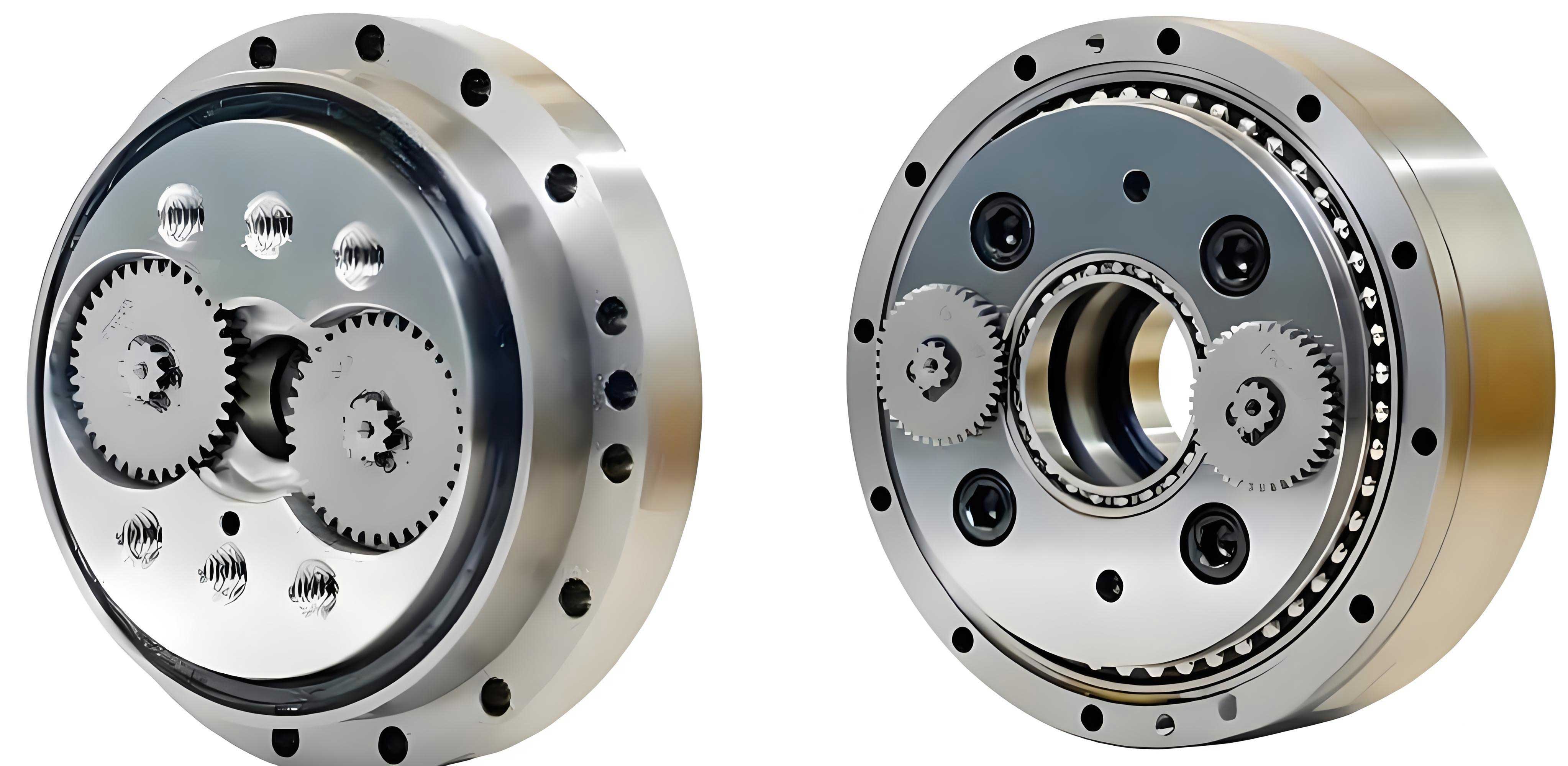
In modern industrial robotics, the Rotate Vector (RV) reducer plays a critical role as a core component in heavy-duty joints such as the robot base, arm, and shoulder. Its performance directly impacts the positioning accuracy, stability, and overall lifespan of industrial robots. However, predicting the remaining useful life (RUL) of RV reducers remains challenging due to the scarcity of run-to-failure data, which is costly and time-consuming to obtain through fatigue life tests. To address this, we propose a novel data-driven framework that integrates multi-domain degradation feature generation and a hybrid deep learning model for accurate RUL prediction of RV reducers. Our approach leverages vibration signals to extract comprehensive features, employs a time-series generative adversarial network (TimeGAN) for data augmentation, and utilizes a convolutional long short-term memory network (C-LSTM) to capture both spatial and temporal dependencies in the degradation process.
The methodology begins with the acquisition of vibration signals from RV reducers during their entire life cycle. We then extract 40 initial features from multiple domains—time domain, time-frequency domain, and trigonometric functions—to comprehensively characterize the health state of the RV reducer. These features are evaluated for monotonicity using trendability indices, and redundant features are eliminated through correlation-based clustering to construct a robust performance degradation indicator system. Subsequently, we apply TimeGAN to learn the latent distribution of the multivariate time-series data formed by the selected features. TimeGAN generates synthetic samples that closely mimic the temporal dynamics and probabilistic distribution of real degradation data, effectively expanding the training dataset. Finally, we design a C-LSTM model that combines convolutional neural networks (CNN) for spatial feature extraction and long short-term memory (LSTM) networks for temporal sequence modeling. This hybrid architecture establishes a mapping between degradation features and the remaining life of the RV reducer, enabling precise RUL estimation.
To validate our framework, we conduct extensive experiments on a real RV reducer lifespan testbed. The results demonstrate that TimeGAN-generated virtual data exhibit superior similarity to real data in both time-series trends and distribution metrics compared to traditional generative models like DCGAN. Moreover, the C-LSTM model achieves significantly lower prediction errors—measured by root mean square error (RMSE), mean absolute error (MAE), and mean square error (MSE)—than conventional models such as standalone CNN, LSTM, and fully connected neural networks. By augmenting the training data with synthetic samples, the prediction performance is further enhanced, underscoring the effectiveness of our multi-domain feature generation approach. In this article, we detail each component of the framework, present experimental analyses, and discuss implications for industrial applications.
1. Introduction
RV reducers are precision transmission devices widely used in industrial robots due to their compact size, high reduction ratio, and excellent motion accuracy. As a key element in robotic joints, the health condition of an RV reducer directly affects the reliability and operational safety of the entire system. Predicting the remaining useful life of RV reducers allows for proactive maintenance, reducing downtime and costs. However, obtaining sufficient run-to-failure data for RV reducers is impractical because lifespan tests require substantial resources. Consequently, data-driven RUL prediction methods often suffer from limited training samples, leading to overfitting and poor generalization.
Traditional data-driven approaches for machinery prognostics include model-based methods, which rely on physical degradation models, and pure data-driven techniques, such as artificial neural networks and support vector regression. For complex components like the RV reducer, constructing accurate physical models is difficult; thus, data-driven methods are preferred. Recent advances in deep learning have enabled more sophisticated RUL prediction models that automatically learn degradation patterns from raw sensor data. For instance, convolutional neural networks (CNN) excel at extracting local spatial features, while long short-term memory (LSTM) networks are adept at capturing temporal dependencies. However, these models require large amounts of labeled data to achieve high accuracy, which is a bottleneck for RV reducer applications.
To overcome data scarcity, generative adversarial networks (GANs) have been employed for data augmentation in various fields. Standard GANs, however, are designed for static data and do not account for temporal correlations in time-series data. Time-series generative adversarial networks (TimeGAN) address this limitation by incorporating an autoencoder and adversarial training to preserve temporal dynamics. In our work, we adopt TimeGAN to generate realistic multivariate time-series of degradation features for RV reducers. This augmentation strategy enriches the training dataset, allowing deep learning models to learn more robust representations.
Furthermore, the degradation process of an RV reducer is multifaceted, involving interactions among multiple components such as gears and bearings. Therefore, a single feature may not suffice to describe the health state. We extract a comprehensive set of features from vibration signals across multiple domains and select the most informative ones to form a degradation indicator system. This multi-domain approach ensures that the predictive model captures diverse aspects of degradation.
In summary, our contributions are threefold: (1) We propose a multi-domain degradation feature selection method to construct a concise yet expressive indicator system for RV reducers. (2) We employ TimeGAN for generating high-quality synthetic time-series data that augment the limited real data. (3) We develop a C-LSTM model that leverages both spatial and temporal features for accurate RUL prediction. Experimental results confirm the superiority of our framework over existing methods.
2. Methodology
The overall framework for RV reducer life prediction consists of four main steps: vibration signal acquisition, performance degradation indicator system construction, training data augmentation via TimeGAN, and RUL prediction using C-LSTM. Each step is elaborated below.
2.1 Vibration Signal Acquisition and Feature Extraction
Vibration signals are collected from RV reducers using tri-axial accelerometers mounted on the reducer housing. Signals are sampled periodically throughout the lifespan, capturing the degradation progression. From the raw vibration data, we extract 40 initial features from three domains: time domain, time-frequency domain, and trigonometric domain. The time-domain features include statistical measures such as standard deviation, peak-to-peak value, root mean square, kurtosis, and skewness. Time-frequency features are derived from wavelet packet decomposition and empirical mode decomposition (EMD), providing insights into frequency-band energies and intrinsic mode functions. Trigonometric features, such as the standard deviation of inverse hyperbolic sine and inverse tangent transformations, offer additional nonlinear characteristics.
The complete list of 40 features is summarized in Table 1. Let the vibration signal be denoted as \( V = \{v_1, v_2, \dots, v_N\} \), where \( N \) is the number of samples. For wavelet packet decomposition, the signal is decomposed to the third level, yielding 8 terminal node coefficients. The energy of each node is computed as:
$$ E_j = \sum_{n=1}^{N} |c_j(n)|^2 \Delta t, \quad j=1,2,\dots,8 $$
where \( c_j(n) \) are the wavelet coefficients and \( \Delta t \) is the sampling interval. The energy ratios are then \( F_{18+j} = E_j / \sum_{i=1}^{8} E_i \). For EMD, the signal is decomposed into intrinsic mode functions (IMFs), and the instantaneous energy of the first six IMFs is calculated as:
$$ E_l = \sum_{n=1}^{N} |c_l(n)|^2 \Delta t, \quad l=1,2,\dots,6 $$
where \( c_l(n) \) is the \( l \)-th IMF. The normalized instantaneous energy ratios are \( F_{32+l} = E_l / \sum_{i=1}^{6} E_i \). The trigonometric features are defined as:
$$ \text{SD of IHS} = \sigma(\log(v_n + \sqrt{v_n^2 + 1})) $$
$$ \text{SD of IT} = \sigma\left(\frac{\log(i + v_n) – \log(i – v_n)}{2i}\right) $$
where \( \sigma(\cdot) \) denotes standard deviation and \( i \) is the imaginary unit.
| Domain | Feature Index | Description |
|---|---|---|
| Time Domain | F1 | Standard deviation |
| F2 | Peak-to-peak value | |
| F3 | Average absolute value | |
| F4 | Root mean square | |
| F5 | Waveform factor | |
| F6 | Peak factor | |
| F7 | Impulse factor | |
| F8 | Skewness | |
| F9 | Kurtosis | |
| F10 | Margin factor | |
| Time-Frequency Domain | F11-F18 | Wavelet packet band energies (8 bands) |
| F19-F26 | Wavelet packet band energy ratios (8 ratios) | |
| F27-F32 | IMF instantaneous energies (6 IMFs) | |
| F33-F38 | IMF instantaneous energy ratios (6 ratios) | |
| Trigonometric Domain | F39 | Standard deviation of inverse hyperbolic sine |
| F40 | Standard deviation of inverse tangent |
2.2 Performance Degradation Indicator System Construction
Not all extracted features are equally informative for degradation tracking. Some may lack monotonic trends, while others may be highly correlated. To select the most representative features, we first compute the trendability index for each feature using the Spearman correlation coefficient with time:
$$ \rho_k = \frac{\sum_{l=1}^{L} (T_l – \bar{T})(Y_{l}^k – \bar{Y}^k)}{\sqrt{\sum_{l=1}^{L} (T_l – \bar{T})^2 \sum_{l=1}^{L} (Y_{l}^k – \bar{Y}^k)^2}} $$
where \( T_l \) is the time at the \( l \)-th sampling point, \( Y_{l}^k \) is the value of the \( k \)-th feature at time \( l \), \( L \) is the total number of sampling points, and \( \bar{T} \), \( \bar{Y}^k \) are the means. Features with \( \rho_k > 0.5 \) are considered to have good monotonicity and are retained.
Next, to reduce redundancy among the selected features, we apply correlation-based clustering. The absolute correlation matrix of the features is computed, and clustering is performed using an algorithm that maximizes the PBM index:
$$ \text{PBM}(Q) = \left( \frac{1}{Q} \cdot \frac{C_1}{C_Q} \cdot D_Q \right)^2 $$
where \( Q \) is the number of clusters, \( C_1 \) is a constant, \( C_Q = \sum_{q=1}^{Q} C_q \), \( C_q = \sum_{m=1}^{M} u_{qm} \lambda_{qm} \), and \( D_Q = \max_{i,j} \lambda_{ij} \). Here, \( u_{qm} \) is the membership of feature \( m \) to cluster \( q \), and \( \lambda \) denotes correlation. The optimal \( Q \) is chosen by maximizing PBM. Within each cluster, the feature with the highest trendability index is selected as the typical feature, forming the final degradation indicator system.
For our RV reducer dataset, this process yields four typical features: energy of wavelet packet band 1, energy of wavelet packet band 5, energy ratio of wavelet packet band 3, and instantaneous energy ratio of IMF1. These features exhibit distinct degradation trends and low mutual correlation, effectively capturing the health state of the RV reducer.
2.3 Data Augmentation Using TimeGAN
With limited run-to-failure data, we employ TimeGAN to generate synthetic multivariate time-series that mimic the real degradation features. TimeGAN combines an autoencoder and a generative adversarial network to preserve temporal dynamics. The model includes four components: an embedding function \( e \), a recovery function \( r \), a generator \( g \), and a discriminator \( d \). The input consists of static data \( S \) (e.g., initial conditions) and dynamic data \( X = \{x_1, x_2, \dots, x_T\} \) (the time-series features). The embedding function maps the data to a latent space:
$$ h_S = e_S(s), \quad h_t = e_X(h_S, h_{t-1}, x_t) $$
where \( e_S \) and \( e_X \) are implemented using gated recurrent units (GRU). The recovery function reconstructs the data from the latent space:
$$ \hat{s} = r_S(h_S), \quad \hat{x}_t = r_X(h_t) $$
The generator produces synthetic latent vectors from random noise:
$$ \tilde{h}_S = g_S(z_S), \quad \tilde{h}_t = g_X(\tilde{h}_S, \tilde{h}_{t-1}, z_t) $$
where \( g_X \) is implemented with LSTM networks. The discriminator evaluates whether latent vectors are real or generated:
$$ y_S = d_S(h_S), \quad y_t = d_X(h_t, u_t) $$
where \( u_t \) represents forward and backward hidden states.
TimeGAN is trained by minimizing a combined loss function that includes reconstruction loss \( L_R \), unsupervised adversarial loss \( L_U \), and supervised loss \( L_S \):
$$ L_R = \mathbb{E}_{s, x_{1:T} \sim p} \left[ \| s – \hat{s} \|_2 + \sum_{t=1}^{T} \| x_t – \hat{x}_t \|_2 \right] $$
$$ L_U = \mathbb{E}_{s, x_{1:T} \sim p} \left[ \log y_S + \sum_{t=1}^{T} \log y_t \right] + \mathbb{E}_{z_S, z_{1:T} \sim p_z} \left[ \log (1 – \tilde{y}_S) + \sum_{t=1}^{T} \log (1 – \tilde{y}_t) \right] $$
$$ L_S = \mathbb{E}_{s, x_{1:T} \sim p} \left[ \sum_{t=1}^{T} \| h_t – g_X(h_S, h_{t-1}, z_t) \|_2 \right] $$
The joint training ensures that the generated sequences are both statistically similar and temporally coherent with the real data.
2.4 RUL Prediction with C-LSTM Model
To predict the remaining useful life of the RV reducer, we design a hybrid neural network called C-LSTM, which integrates CNN and LSTM layers. The CNN layers extract spatial features from the multivariate time-series, while the LSTM layers capture long-term temporal dependencies. The model architecture is shown in Figure 3, with detailed parameters in Table 2.
The input to the C-LSTM model is a window of sequential data from the degradation features (real and augmented). Each window has a length of 200 time steps and includes the four typical features. The CNN component consists of four 1D convolutional layers with ReLU activation and batch normalization. The LSTM component comprises two LSTM layers with 64 units each. A residual connection is added to facilitate gradient flow. The output layer is a fully connected layer that produces the RUL estimate for each time step.
The model is trained using the augmented dataset (real data plus TimeGAN-generated data) to learn the mapping from degradation features to RUL. The loss function is mean squared error (MSE), and optimization is performed using Adam. During testing, the model takes unseen feature sequences and outputs predicted RUL values, which are compared with the actual RUL for evaluation.
| Layer | Number of Kernels/Units | Kernel Size/Stride | Output Size | Zero Padding |
|---|---|---|---|---|
| Input | – | – | 200 × 4 | – |
| Conv1D 1 | 32 | 3 × 1 / 1 | 200 × 32 | Yes |
| Conv1D 2 | 32 | 3 × 1 / 1 | 200 × 32 | Yes |
| Conv1D 3 | 64 | 3 × 1 / 1 | 200 × 64 | Yes |
| Conv1D 4 | 64 | 3 × 1 / 1 | 64 × 1 | Yes |
| LSTM 1 | 64 | – | 64 × 1 | – |
| LSTM 2 | 64 | – | 64 × 1 | – |
| Output | 1 | – | 1 × 1 | – |
3. Experimental Validation
We validate the proposed framework using a real RV reducer lifespan testbed. The testbed comprises an RV reducer (model CORT40E-121) driven by a servo motor, with a swinging arm and load to simulate operational conditions. Vibration signals are collected every 0.5 hours using a tri-axial accelerometer mounted on the reducer housing, with a sampling frequency of 5000 Hz. The test runs until the RV reducer fails, resulting in 575 hours of data (1150 sampling points). Post-failure analysis reveals that the failure is caused by bearing damage in the crank shaft support, with balls脱落 and cracks in the inner race and cage.
3.1 Degradation Indicator System for the RV Reducer
From the vibration signals (axial direction), we extract the 40 initial features. The trendability indices are computed, and 21 features with \( \rho_k > 0.5 \) are retained. Clustering analysis using the PBM index identifies four optimal clusters. The typical features selected are: energy of wavelet packet band 1 (F11), energy of wavelet packet band 5 (F15), energy ratio of wavelet packet band 3 (F21), and instantaneous energy ratio of IMF1 (F33). These features show clear monotonic trends over the lifespan, as illustrated in Figure 9, and are used as the degradation indicator system for subsequent steps.
3.2 Quality of Generated Data from TimeGAN
We train TimeGAN on the real multivariate time-series of the four typical features. The generated synthetic sequences are compared with real data in terms of temporal trends and distribution similarity. For comparison, we also generate data using a deep convolutional GAN (DCGAN). Visual inspection shows that TimeGAN-generated data closely follow the temporal dynamics of real data, whereas DCGAN-generated data exhibit erratic trends. Quantitative metrics, including Fréchet distance and maximum mean discrepancy (MMD), confirm the superiority of TimeGAN. The results are summarized in Tables 3 and 4.
| Feature | DCGAN | TimeGAN |
|---|---|---|
| IMF1 instantaneous energy ratio | 1.2733 | 0.3937 |
| Wavelet packet band 1 energy | 0.9335 | 0.7013 |
| Wavelet packet band 5 energy | 0.9375 | 0.7986 |
| Wavelet packet band 3 energy ratio | 1.1191 | 1.0046 |
| Feature | DCGAN | TimeGAN |
|---|---|---|
| IMF1 instantaneous energy ratio | 0.4344 | 0.2123 |
| Wavelet packet band 1 energy | 0.3430 | 0.2974 |
| Wavelet packet band 5 energy | 0.5164 | 0.4508 |
| Wavelet packet band 3 energy ratio | 0.4586 | 0.3904 |
Lower values indicate better similarity. TimeGAN consistently outperforms DCGAN, demonstrating its ability to generate realistic time-series for RV reducer degradation features.
3.3 Life Prediction Results and Comparative Analysis
We conduct several experiments to evaluate the RUL prediction performance. The real data is split: first 50% for training, last 50% for testing. The C-LSTM model is trained under two conditions: (a) using only real data, and (b) using augmented data (real data plus 24 synthetic sequences from TimeGAN). Prediction results are assessed using RMSE, MAE, and MSE.
The prediction curves show that augmented data significantly improves accuracy, especially in the early and middle stages of degradation. Quantitative results are presented in Table 5. With data augmentation, RMSE decreases by 81.20%, MAE by 79.30%, and MSE by 96.47%, highlighting the effectiveness of TimeGAN for enhancing model training.
| Metric | Without Augmentation | With Augmentation | Improvement |
|---|---|---|---|
| RMSE | 0.23979 | 0.04507 | 81.20% |
| MAE | 0.17472 | 0.03615 | 79.30% |
| MSE | 0.05750 | 0.00203 | 96.47% |
We further optimize hyperparameters of the C-LSTM model, including the number of convolutional layers, kernel size, and stride. The best configuration is 4 convolutional layers, kernel size 3×1, and stride 1, as it yields the lowest errors (Table 6).
| Configuration | RMSE | MAE | MSE |
|---|---|---|---|
| 2 layers, kernel 3×1, stride 1 | 0.05981 | 0.04381 | 0.00358 |
| 4 layers, kernel 3×1, stride 1 | 0.04507 | 0.03615 | 0.00203 |
| 6 layers, kernel 3×1, stride 1 | 0.07251 | 0.05571 | 0.00526 |
To demonstrate the superiority of C-LSTM, we compare it with baseline models: CNN, LSTM, and fully connected neural network (FCNN), all trained on augmented data. The results in Table 7 show that C-LSTM achieves the lowest errors, benefiting from its hybrid architecture that captures both spatial and temporal patterns.
| Model | RMSE | MAE | MSE |
|---|---|---|---|
| CNN | 0.30247 | 0.19665 | 0.09149 |
| LSTM | 0.07486 | 0.05709 | 0.00560 |
| FCNN | 0.24371 | 0.17528 | 0.05939 |
| C-LSTM (proposed) | 0.04507 | 0.03615 | 0.00203 |
Additionally, we validate the feature selection method by comparing it with principal component analysis (PCA). Using PCA to reduce the 40 features to 4 dimensions and then applying the same TimeGAN and C-LSTM pipeline yields higher errors (Table 8), confirming that our trendability and clustering-based selection better preserves degradation information for RV reducers.
| Feature Method | RMSE | MAE | MSE |
|---|---|---|---|
| PCA (4 components) | 0.05122 | 0.03872 | 0.00262 |
| Proposed selection | 0.04507 | 0.03615 | 0.00203 |
4. Conclusion
In this work, we present a comprehensive framework for predicting the remaining useful life of RV reducers by addressing the data scarcity problem through multi-domain degradation feature generation. Our approach extracts a wide range of features from vibration signals, selects the most informative ones via trendability analysis and clustering, and employs TimeGAN to generate realistic synthetic time-series data. The augmented dataset is then used to train a hybrid C-LSTM model that effectively learns spatial and temporal degradation patterns. Experimental results on a real RV reducer lifespan dataset demonstrate that TimeGAN generates high-quality virtual data superior to DCGAN, and the C-LSTM model outperforms traditional deep learning models in RUL prediction accuracy. Data augmentation reduces prediction errors by over 80%, underscoring its value for practical applications.
However, limitations exist. TimeGAN may not fully capture abrupt changes in degradation trends, and the C-LSTM model could be improved for long-term dependency modeling. Future work will focus on enhancing the generative model with adaptive feature compression and incorporating attention mechanisms into the prediction network to better handle nonlinear degradation dynamics. Overall, our framework provides a viable solution for RV reducer prognostics, with potential extensions to other critical machinery components in industrial robotics.